Robots with fewer motors than joints¶

Some robots have joints that no motor drives: a finger whose last joint follows a spring, a soft arm whose tendons bend it in fewer ways than it can bend. A virtual spring on such a robot asks for torques that the motors cannot all give. In this tutorial we control a planar arm with three joints and two motors, see what is lost, and compare the two ways the library renders the torques, with and without a correction that keeps the arm passive. If you only want to know which controller to take, read Choosing at the end.

The arm¶

The arm moves in the vertical plane. Motors drive joints 1 and 3; joint 2 is passive, with a torsional spring and a damper of its own. planar.arm builds the robot and planar.add_dynamics gives it gravity and the passive joint’s spring and damper.

import numpy as np
import matplotlib.pyplot as plt
import virtualmodelcontrol as vmc
from virtualmodelcontrol import viz
from virtualmodelcontrol.control import underactuated as ua
from virtualmodelcontrol.robots import planar

arm = planar.add_dynamics(planar.arm("three-link"))
kin = vmc.Kinematics(arm)
B = arm.actuation.params["B"].value  # the motors' input matrix
print(B)

[[1. 0.]
 [0. 0.]
 [0. 1.]]

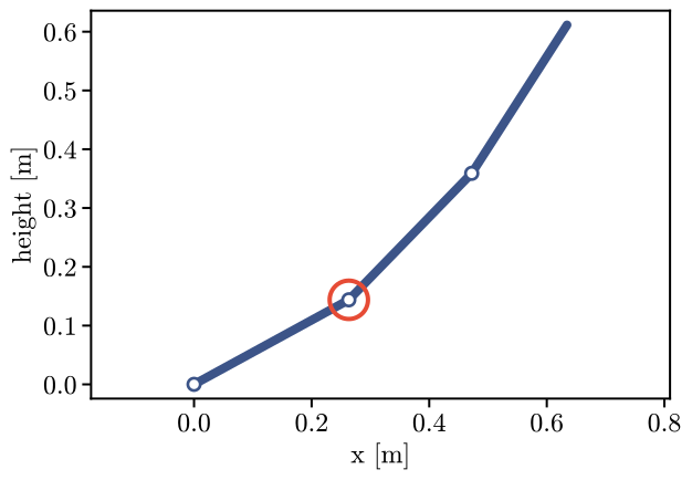
The motor torques \(u\) reach the joints as \(\tau = B u\). Joint 2 gets nothing from them. This is the actuation models.Underactuated; Direct is the case with a motor on every joint.

What the motors can give¶

A virtual spring and damper on the tip give a force \(F\), and the torque it asks of the joints is \(J^\top F\). The motors give the part of it they can reach, \(B B^+ J^\top F\), with \(B^+ = (B^\top B)^{-1} B^\top\). What is left is the torque defect \(E J^\top F\), with \(E = I - B B^+\) the projector on the torques no motor gives. Here \(E\) keeps only joint 2.

q = np.array([0.5, 0.3, 0.2])
J = kin.jacobian(q, "tip")[:2]  # the tip in the plane: x and y
F = np.array([2.0, -1.0])  # [N]
lost = ua.defect(B, J, F)  # [N·m]
asked = J.T @ F
print("asked", asked, "lost", lost)

asked [-1.85732904 -1.30639895 -0.66697328] lost [ 0.         -1.30639895  0.        ]

The defect is -1.31 N·m at joint 2, the whole of the -1.31 N·m that the force asked of it. Joint 2 moves the tip along one direction only, and a force at the tip is realized in full when it asks nothing of joint 2: when it is perpendicular to that direction, so that its torque at joint 2 is zero. These forces are the feasible set, here a line:

basis = ua.feasible(B, J)  # columns: forces the motors give in full
print(basis.T, ua.defect(B, J, 3.0 * basis[:, 0]))

[[0.62160997 0.78332691]] [ 0.00000000e+00 -2.22044605e-16  0.00000000e+00]

The basis is that perpendicular direction, and the defect of a force along it is zero.

A spring of the controller can pull the tip only along such a direction without error; any other pull is partly absorbed by the passive joint, which moves until its own spring balances what is left.

A reach, rendered two ways¶

The controller is a spring from the tip to a goal, a damper, and the compensation of the arm’s weight. ua.controller(compiled, base, correction=None, *, gravity=False, tank=1.0) builds it, and base chooses how its torques are rendered:

• "naive" sends the motors \(u = B^+ J^\top F\), the least-squares torques at the measured state. It needs the whole state \((q, v)\), passive joint included, so it is a StateController: it reads \(q\) and \(v\) of the measurement, not the motors’.

• "frozen" evaluates the same law with the passive joint held at its rest angle, whatever it does. It needs the motors only, and its torque is the exact gradient of a potential. With gravity=True it holds the passive joint where its spring balances the arm’s own weight instead of at the rest angle.

def reach(robot, compensate=True, stiffness=150.0):
    tip = robot.point("tip")
    ctrl = vmc.Mechanism("ctrl")
    ctrl.add("reach", vmc.LinearSpring(tip - [0.45, 0.15, 0.0], stiffness))
    ctrl.add("damp", vmc.LinearDamper(tip, 25.0))
    if compensate:
        ctrl.add("gravity", vmc.GravityCompensation(robot))
    return vmc.compile(vmc.VirtualMechanismSystem(robot, ctrl))

def run(compiled, base, correction=None, gravity=False, T=4.0):
    controller = ua.controller(compiled, base, correction, gravity=gravity)
    plant = vmc.sim.ModelPlant(arm, q0=[0.3, 0.3, 0.3], max_step=1e-4)
    log = vmc.sim.run(plant, controller, vmc.sim.SimClock(5e-4), T=T)
    return log.arrays()

compiled = reach(arm)
runs = {"naive": run(compiled, "naive"),
        "frozen": run(compiled, "frozen"),
        "frozen, gravity": run(compiled, "frozen", gravity=True)}

def tip_error(rows):
    tips = np.array([kin.position(x, "tip")[:2] for x in rows["q"][::10]])
    return np.linalg.norm(tips - [0.45, 0.15], axis=1)  # [m]

fig, ax = plt.subplots()
for name, rows in runs.items():
    ax.plot(np.ravel(rows["t"])[::10], 1000 * tip_error(rows), label=name)
ax.set_xlabel("time [s]")
ax.set_ylabel("distance to the goal [mm]")
ax.legend(fontsize=18);

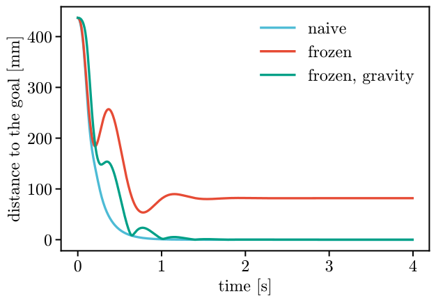
With the weight compensated, the naive controller settles on the goal, within 6.4e-09 mm. The plain frozen controller stops 82 mm short: it renders the force as if the passive joint were at its rest angle, but the joint carries the weight of the links beyond it and sags. With gravity=True it knows that and settles within 2.9e-05 mm. Without the compensation, the arm’s own weight pulls the tip away, and the controllers end 75 mm from the goal (naive, and frozen with gravity=True) and 148 mm (plain frozen). Where the passive joint is at rest and carries nothing, naive and frozen send the same torques.

Keeping the arm passive¶

The naive torque is not the gradient of anything, so a controller built on it can put energy into the arm that no damper took out. Two output stages of the controller limit that. The passive correction removes the least torque that keeps the power the motors inject below the power the arm’s own dampers dissipate, \(\dot\theta^\top u \le P_D\), with \(\dot\theta\) the motor rates and \(P_D\) the power of those dampers. The tank correction lets the motors inject more while a tank, which starts with a budget of energy and is refilled by the dissipation, is not empty. Both read the passive joint’s velocity, so the measurement must hold \(q\) and \(v\) (a simulated plant reports them).

dynamics = vmc.compile_dynamics(arm)
p = dynamics.live_values()

def energy(rows):  # [J], kinetic and stored energy of the arm itself
    return np.array([sum(float(e) for e in dynamics.energy(q, v, p, 0.0))
                     for q, v in zip(rows["q"][::10], rows["v"][::10])])

corrected = {name: run(compiled, "naive", name)
             for name in (None, "passive", "tank")}
fig, ax = plt.subplots()
for name, rows in corrected.items():
    ax.plot(np.ravel(rows["t"])[::10], energy(rows),
            label=name or "no correction")
ax.set_xlabel("time [s]")
ax.set_ylabel("energy of the arm [J]")
ax.legend(fontsize=18);

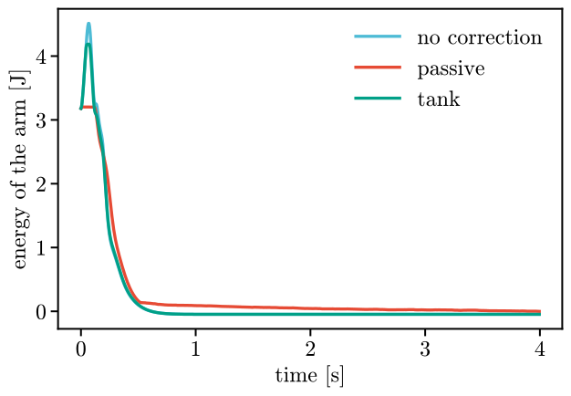
Without a correction the arm gains up to 1.33 J from the controller. With the passive correction it gains 0.023 J at most, the rounding of the control period (the guarantee holds in continuous time and the gain falls with the period). With the tank it gains 1.01 J, the budget it started with (the default tank=1.0 J of ua.controller). The frozen controller needs no correction for its own torque, which is a gradient.

A force along a direction¶

DirectionalForce makes the arm push with a chosen force along one direction by adapting one number of the stiffness. It keeps \(K' = K + s\,n n^\top\), which is symmetric for every \(s\), and moves \(s\) to the value that makes the force the motors realize along \(n\) equal the wanted one, without ever losing \(K' \succ 0\). The spring’s stiffness must be a live \(3 \times 3\) matrix: the spring acts on the tip in 3D, \(z\) included, although the arm moves in a plane. Here the arm is held at a pose and asked for 3 N along \(x\). rate is the share of the way to the right \(s\) that it covers per second, and step(controller, q, v, dt) takes the state the law is evaluated at and the time step, 10 ms here:

compiled = reach(arm, stiffness=150.0 * np.eye(3))
controller = ua.controller(compiled, "naive")
tracker = ua.DirectionalForce(controller, "tip", "ctrl.reach.stiffness",
                              [1, 0, 0], 3.0, rate=2.0)
q, v = np.array([0.5, 0.3, 0.2]), np.zeros(3)
motors = B.T
hold = vmc.Signals(0.0, motor_position=motors @ q,
                   motor_velocity=motors @ v, q=q, v=v)
controller.reset(0.0, hold)
controller.step(0.0, hold)
pushed = []
for _ in range(500):
    tracker.step(controller, q, v, 1e-2)
    pushed.append(tracker.reading)
fig, ax = plt.subplots()
ax.plot(1e-2 * np.arange(500), pushed)
ax.axhline(3.0, color=viz.PALETTE[1], ls="--")
ax.set_xlabel("time [s]")
ax.set_ylabel("force along $x$ [N]");

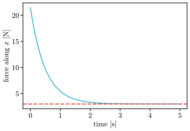
The force settles at 3.00 N. The stiffness along \(x\) changed by \(s\) = 153.1 N/m, and the smallest eigenvalue of \(K'\) is 150.0 N/m, still positive. In your own loop, call tracker.step after each control step with the state the law was evaluated at.

Harder cases¶

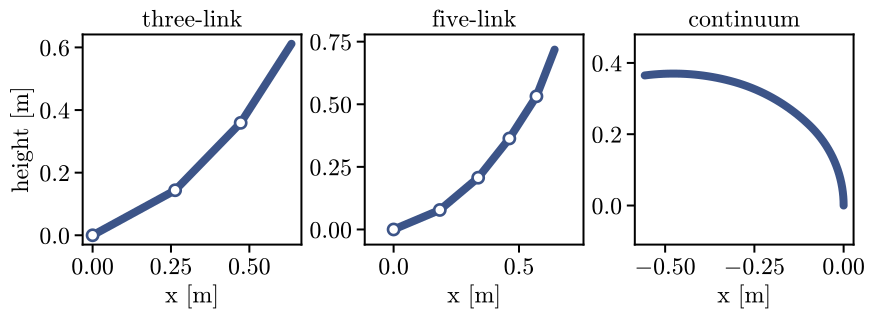
The five-link arm has joints 2, 3 and 4 passive; the continuum arm has three bending sections and two tendons, so the bending of section 2 against 3 has no motor. Both are built the same way and compile with the same controllers.

robots = {"three-link": planar.arm("three-link"),
          "five-link": planar.arm("five-link"),
          "continuum": planar.continuum()}
for name, robot in robots.items():
    n = robot.model.space.nq
    Bn = robot.actuation.params["B"].value
    rank = round(float(np.trace(ua.projector(Bn))))  # rank of E
    print(f"{name:11s} {n} coordinates, {Bn.shape[1]} motors, "
          f"{rank} passive directions")

three-link  3 coordinates, 2 motors, 1 passive directions
five-link   5 coordinates, 2 motors, 3 passive directions
continuum   3 coordinates, 2 motors, 1 passive directions

When the passive joint is not measured¶

The naive controller needs the angle and the rate of every joint, and the encoders give the two motors’ only. A Kalman filter on the arm’s own model can estimate the rest: the passive joint moves the other two through the coupling, and the filter reads it from them. encoder knows that this arm has fewer motors than joints. It reports what the motors see, \(\theta = B^\top q\), as combinations of \(q\) (the measurement’s matrix), not as a reading of \(q\), so the passive joint is left to the model. Each period the loop updates the filter with the encoders, hands the estimate to the controller as the signals q and v, and predicts the next period from the torques it sent.

from virtualmodelcontrol.estimation import Encoders, KalmanFilter

def estimated_run(stiffness, Q, T=3.0, dt=5e-4, estimate=True):
    compiled = reach(arm, stiffness=stiffness)
    onboard = ua.controller(compiled, "naive")
    plant = vmc.sim.ModelPlant(arm, q0=[0.5, -0.3, 0.8], max_step=1e-4)
    encoders = Encoders(arm, noise=1e-4, rate_noise=1e-3)
    kf = KalmanFilter(compiled.system, dt, Q=Q)
    kf.reset([0.5, -0.1, 0.8])  # the passive joint starts 0.2 rad off
    onboard.reset(0.0, plant.read())
    rows = []
    try:
        for _ in range(round(T / dt)):
            theta, rate = encoders.read(plant.q, plant.v)
            kf.update([kf.encoder(theta, rate, 1e-8, 1e-6)])  # variances
            seen = vmc.Signals(plant.t, motor_position=theta,
                               motor_velocity=rate, q=kf.q, v=kf.v)
            if not estimate:  # the controller reads the true state instead
                seen = plant.read()
            cmd = onboard.step(plant.t, seen)
            plant.write(cmd)
            plant.advance(dt)
            kf.predict(cmd["motor_torque"], plant.t)
            rows.append([plant.t, *plant.q, *kf.q])
    except np.linalg.LinAlgError:  # the covariance is no longer a number
        pass
    return np.array(rows), kf.rejected_total

Process noise Q says how far the filter trusts its model over one period. We run the arm, with a spring of 30 N/m to the goal, from near the goal and with the passive joint’s estimate 0.2 rad off, at the default \(Q = 10^{-6}\) and at \(Q = 10^{-3}\):

estimates = {"Q = 1e-6": estimated_run(30.0, 1e-6),
             "Q = 1e-3": estimated_run(30.0, 1e-3)}

def tip_gap(rows):  # [m]
    tips = np.array([kin.position(q, "tip")[:2] for q in rows[::20, 1:4]])
    return np.linalg.norm(tips - [0.45, 0.15], axis=1)

fig, axes = plt.subplots(1, 2, figsize=(11, 4.2), sharey=True)
for ax, (name, (rows, _)) in zip(axes, estimates.items()):
    ax.plot(rows[:, 0], rows[:, 2], label="passive joint")
    ax.plot(rows[:, 0], rows[:, 5], "--", label="estimate")
    ax.set_title(name)
    ax.set_xlabel("time [s]")
axes[0].set_ylabel("angle [rad]")
axes[1].legend(fontsize=18);

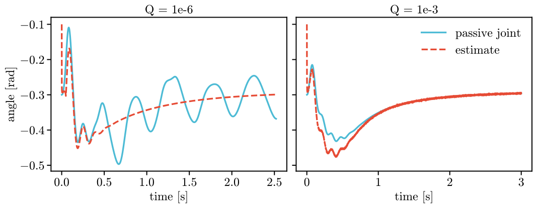
With \(Q = 10^{-3}\) the estimate reaches the passive joint in 20 ms, then stays within 55 mrad of it through the first swing, within 5 mrad from 1.0 s on, and within 3.0 mrad over the last second. The tip ends 11.0 mm from the goal, which is where the controller on the true state ends (the gravity compensation is not exact on the passive joint). With the default \(Q\) the filter believes its model to the last digit. In the first swing the model is wrong by more than that, the gate throws the readings out, and it goes on throwing them out: 4942 of the 5040 it saw. The estimate then runs on the model alone, and its covariance grows until the filter breaks. A count of rejected readings that rises at every step (kf.rejected_total) means the filter has lost its sensors: raise Q, widen the gate of KalmanFilter (40 by default) or pass gate=None.

The estimate costs gain. With the spring at 150 N/m instead of the 30 N/m of these runs, the same filter loses the encoders in the first swing (5681 readings thrown out) and the arm runs away from the goal: a stiff controller moves the arm faster than the filter follows. Soften the controller, or use "frozen", which needs the motors only.

Take it to the robot¶

On the robot the same law runs in the loop that talks to the motors, with nothing from vmc.sim. The loop builds the controller once, and each period it passes the reading to step and sends back the torques. The frozen controller needs only the motors’ angles and rates; the corrections also read \(q\) and \(v\), from a plant that reports them or from an estimate of the unmeasured joints (see the section above). Here is one period with a made-up reading:

compiled = reach(arm)
onboard = ua.controller(compiled, "frozen", "tank", tank=0.5)  # [J]
reading = vmc.Signals(
    0.0, motor_position=[0.3, 0.3], motor_velocity=[0.0, 0.0],
    q=[0.3, 0.3, 0.3], v=[0.0, 0.0, 0.0])
onboard.reset(0.0, reading)
onboard.step(0.0, reading)["motor_torque"]  # [N·m]

array([1.2958308 , 2.72329157])

Choosing¶

• Start with "frozen", with gravity=True if the arm carries weight: it needs only the motors, its torque is a gradient, and it agrees with the naive one where the passive joints rest.

• Take "naive" when the whole state is measured or estimated well and you want the force the spring asks for even away from the passive joints’ rest.

• Add "passive" when the arm must never gain energy, and "tank" to allow short bursts up to a budget. A correction removes torque, so it can slow the reach; set tank to what the task needs.

• The laws and estimators that read a controller’s motors (ForceTracking, StiffnessTracking, PositionRegulation, HoldingGoals, ContactForce, TaskStiffness) refuse a StateController, which is what "naive" and "frozen" with gravity=True give, with a ValueError. Plain "frozen" is a VMCController and works with them; for a force on an underactuated arm use DirectionalForce.

• gravity=True holds the passive joints where their springs balance the arm’s weight, not at the rest angle: the right reference for an arm that hangs or reaches out. The weight itself is compensated by a GravityCompensation in the controller, as for any robot.

• planar.arm(rest=...) sets the passive joints’ rest angles; the frozen controller and the passive spring read them from the same place.