Plan periodic motions and virtual states¶

In this tutorial the optimizer plans motions that repeat, with a period it finds itself, and motions of a controller that has states of its own. A mass on a spring has a known answer to compare with.

import numpy as np
import matplotlib.pyplot as plt
import virtualmodelcontrol as vmc
from virtualmodelcontrol import optimization as opt

A periodic motion with a free period¶

A gait, a swing or a stroke repeats, so we plan one cycle and ask that it closes on itself. Collocation(periodic=True) makes the last node equal to the first (q and v) and leaves the first node free: q0 is only the solver’s starting guess. With free_time=(lower, upper) the horizon is an unknown too, within these bounds, and horizon is where the solver starts: the period is found, not given.

The simplest case has a known answer. A mass on a spring, with nothing driving it, swings with the period \(2\pi\sqrt{m/k}\). We pin the amplitude and ask for the orbit:

mass, stiff = 1.0, 4.0  # [kg], [N/m]
robot = vmc.Mechanism("swing", model=vmc.models.JointSpace(1, unit="m"))
pos = robot.joint(0)
robot.add("mass", vmc.Inertance(pos, mass))
robot.add("spring", vmc.LinearSpring(pos, stiff))
free_swing = vmc.VirtualMechanismSystem(robot, vmc.Mechanism("none"))

amp, nodes = 0.3, 41  # [m]
swing = opt.Problem(free_swing)
swing.add(opt.Collocation(
    [amp], 3.0, nodes, periodic=True, free_time=(2.0, 4.5),
    scheme="hermite-simpson"))
swing.add(opt.Bound(pos, amp, amp, t_from=0.0, t_to=0.0, name="start"))
swing.add(opt.Cost(pos, name="small"));

Bound reaches the first node here, since a periodic motion has no fixed start. A window such as t_from=0.0, t_to=0.0 picks its nodes by their times at the starting horizon, and keeps them when the horizon changes.

The amplitude is pinned at the first node, but a swing that is wider and passes through the pin also repeats. The small Cost on the position chooses the narrowest orbit, the one that turns at the pin. A periodic orbit is also hard to find from a robot at rest, so we start the solver from a guess of it, a cosine of the wrong period:

start = 3.0  # [s]
t0 = np.linspace(0.0, start, nodes)
guess = {"q": amp * np.cos(2 * np.pi * t0 / start)[:, None],
         "horizon": start}
orbit = swing.solve(warm_start=guess)
spring_period = 2 * np.pi * np.sqrt(mass / stiff)  # [s]
print(orbit.status, orbit.iterations, orbit.horizon, spring_period)

Solve_Succeeded 3 3.1415969061978117 3.141592653589793

The solver ended with Solve_Succeeded after 3 iterations, from a horizon of 3.0 s. It found a period of 3.1416 s, where \(2\pi\sqrt{m/k}\) is 3.1416 s: they differ by 1.4e-06 of the period, the error of Hermite-Simpson with 41 nodes. orbit.horizon is the horizon it found, and orbit.t the nodes’ times on it.

tt = np.linspace(0.0, spring_period, 200)

fig, ax = plt.subplots()
ax.plot(tt, amp * np.cos(2 * np.pi * tt / spring_period), label="exact")
ax.plot(orbit.t, orbit.q[:, 0], "o", ms=5, label="periodic plan")
ax.plot(t0, guess["q"][:, 0], ":", color="gray", label="first guess")
ax.set_xlabel("time [s]")
ax.set_ylabel("position [m]")
ax.legend(loc="lower left", fontsize=18);

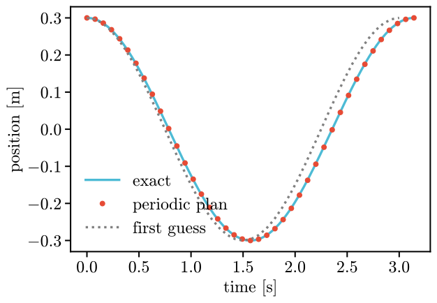
The orbit closes at the period of the spring, and the dotted guess, which closes at 3 s, does not.

A controller that keeps time¶

A controller can repeat too. Its reference is a function of time, vmc.Time(), with the period in a Param. The orbit repeats if the horizon is that period, and opt.Period(name) ties the two: it holds the horizon equal to the Param, which can be free like any other. Here a spring pulls the swinging mass towards a goal that moves as \(a\cos\omega t + b\sin\omega t\), with \(a\), \(b\) and the period free. Their scope="episode" says that they change between runs, not during one (Parameters). We ask for the orbit through the amplitude \(0.3\) m that costs the least effort:

import casadi as ca

period = vmc.Param("period", 3.0, unit="s", bounds=(1.5, 6.0),
                   scope="episode")
cos = vmc.Param("cos", 0.0, unit="m", scope="episode")
sin = vmc.Param("sin", 0.0, unit="m", scope="episode")


def circle(t, period, cos, sin):  # repeats every `period` seconds
    phase = 2 * np.pi * t / period
    return cos * ca.cos(phase) + sin * ca.sin(phase)


rub = 0.8  # friction [N s/m]
rubbed = vmc.Mechanism("rubbed", model=vmc.models.JointSpace(1, unit="m"))
pos2 = rubbed.joint(0)
rubbed.add("mass", vmc.Inertance(pos2, mass))
rubbed.add("spring", vmc.LinearSpring(pos2, stiff))
rubbed.add("friction", vmc.LinearDamper(pos2, rub))

moving = vmc.Custom(circle, [vmc.Time()], dim=1, unit="m", params={
    "period": period, "cos": cos, "sin": sin})
pull = vmc.Mechanism("pull")
pull.add("spring", vmc.LinearSpring(pos2 - moving, 10.0))
keeps_time = vmc.VirtualMechanismSystem(rubbed, pull)

least = opt.Problem(keeps_time)
least.add(opt.Collocation(
    [amp], 3.0, nodes, periodic=True, free_time=(1.5, 6.0),
    scheme="hermite-simpson"))
least.free("pull.spring.period", "pull.spring.cos", "pull.spring.sin")
least.add(opt.Period("pull.spring.period"))
least.add(opt.Bound(pos2, amp, amp, t_from=0.0, t_to=0.0, name="start"))
least.add(opt.Effort(1.0))
best = least.solve()
print(best.status, best.horizon, best.params["pull.spring.period"])

Solve_Succeeded 3.205699996616091 3.205699996616091

The force the controller must give is \(m\ddot x + c\dot x + kx\). For \(x = a\cos\omega t\) the effort over a period is \(\frac{T}{2}a^2\left((k - m\omega^2)^2 + c^2\omega^2\right)\) with \(T = 2\pi/\omega\), and its minimum in \(T\) is at the positive root \(s\) of \(3m^2s^2 + (c^2 - 2km)s - k^2 = 0\), with \(s = \omega^2\):

m, c, k = mass, rub, stiff
s = max(np.roots([3 * m**2, c**2 - 2 * k * m, -(k**2)]).real)
period_best = 2 * np.pi / np.sqrt(s)


def effort(T):  # [N^2 s] over one period, for x = amp cos(2 pi t / T)
    w = 2 * np.pi / T
    return T / 2 * amp**2 * ((k - m * w**2) ** 2 + (c * w) ** 2)


Ts = np.linspace(1.5, 6.0, 200)
fig, ax = plt.subplots()
ax.plot(Ts, effort(Ts), label="closed form")
ax.plot([best.horizon], [best.cost], "o", ms=10, label="found")
ax.axvline(spring_period, color="gray", linestyle=":")
ax.set_xlabel("period [s]")
ax.set_ylabel(r"effort [N$^2$ s]")
ax.legend(loc="upper right", fontsize=18);

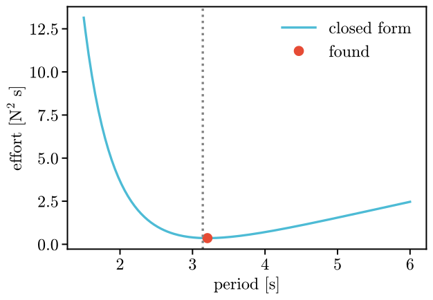
The solver found a period of 3.206 s and an effort of 0.3583 N\(^2\) s in 18 iterations; the closed form says 3.206 s. It is not the period of the spring alone (3.142 s, the dotted line): friction moves it. best.params holds the goal’s \(a\) and \(b\) and the period, and apply puts them into a controller like any other result.

Good to know about periodic problems and a free horizon:

• A guess of the orbit. From a robot at rest the solver may not find a swing, on a coarse grid especially. Give solve a warm_start with the orbit’s q (and v, a) and the horizon.

• Windows. Cost and Bound choose their nodes by the times of the starting horizon and keep those nodes whatever the horizon becomes. Effort and Cost integrate with the horizon that is found. To write your own term, use trajectory.dt, trajectory.times and trajectory.horizon: they are numbers for a fixed horizon and expressions of the free one otherwise (a cost on the time itself is weight * trajectory.horizon).

• Equations and unknowns. The solver needs no more equations than unknowns. A swing with a fixed horizon that pins its start by an equality has one too many: pin it from one side (Bound(pos, amp, None, ...)) and let the cost close the bound, or free the horizon.

• Not together. initial and transition blend two controllers by the nodes’ times, which must be numbers: they go with neither periodic nor free_time. (The swap and the transition are in Optimizing a virtual mechanism.)

A controller with virtual states¶

A controller can have states of its own, such as a virtual mass that the robot is tied to, or the flywheel of a gait. The plan then has them as unknowns too, with the controller’s own dynamics, and nothing changes in the problem: Collocation, Equilibrium and Shooting find the states in the controller. As an example, a mass is held by a spring to a virtual mass \(z\), and \(z\) is pulled by a spring to a goal. We free the goal, and ask for the mass to be at 1 m after 2 s:

line = vmc.Mechanism("line", model=vmc.models.JointSpace(1, unit="m"))
pos3 = line.joint(0)
line.add("mass", vmc.Inertance(pos3, 1.0))
line.add("friction", vmc.LinearDamper(pos3, 1.0))

goal = vmc.Param("goal", 1.0, bounds=(-5.0, 5.0), unit="m", scope="stage")
follower = vmc.Mechanism("follower")
z = follower.add_state("z", 1, unit="m")  # the virtual mass
follower.add("inertia", vmc.Inertance(z, 0.5))
follower.add("link", vmc.LinearSpring(pos3 - z, 10.0))
follower.add("anchor", vmc.LinearSpring(z - vmc.Ref("goal", 1, goal), 4.0))
follower.add("damper", vmc.LinearDamper(z, 2.0))
tied = vmc.VirtualMechanismSystem(line, follower)

reach = opt.Problem(tied)
reach.add(opt.Collocation([0.0], 3.0, 31, scheme="hermite-simpson"))
reach.add(opt.Bound(pos3, 1.0, 1.0, t_from=2.0, t_to=2.0, name="arrive"))
reach.add(opt.Effort(0.1))
reach.free("follower.anchor.goal")
tied_plan = reach.solve()
print(tied_plan.status, tied_plan.params, tied_plan.z.shape)

Solve_Succeeded {'follower.anchor.goal': array(0.94611334)} (31, 2)

plan.z holds the virtual state at every node, the position of \(z\) and then its velocity, like q and v for the robot. The state starts where the controller starts, which is the initial= of add_state (0 here), at rest; Collocation(z0=...) starts it elsewhere. We check the plan by applying the goal and running the closed loop on a simulation with a finer step:

tied_plan.apply(tied)
check = vmc.sim.rollout(tied, [0.0], 3.001, 0.001, max_step=0.001,
                      integrator="rk4")
rows = np.round(tied_plan.t / 0.001).astype(int)
error = np.abs(tied_plan.q[:, 0] - check["q"][rows, 0]).max()

fig, ax = plt.subplots()
ax.plot(tied_plan.t, tied_plan.q[:, 0], label="mass")
ax.plot(tied_plan.t, tied_plan.z[:, 0], label="virtual mass")
ax.plot(check["t"], check["q"][:, 0], "k:", label="simulation")
found = tied_plan.params["follower.anchor.goal"]
ax.axhline(found, color="gray", linestyle="--")
ax.set_xlabel("time [s]")
ax.set_ylabel("position [m]")
ax.legend(loc="lower right", fontsize=18);

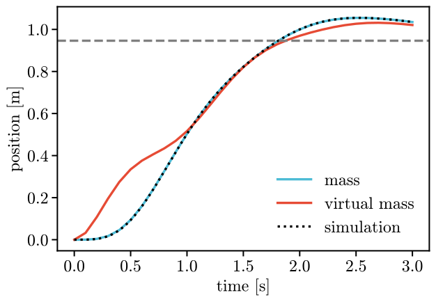
The goal that does it is 0.946 m: the mass passes 1 m at 2 s and overshoots the goal. The plan agrees with the simulation to 0.5 mm. A controller advances its virtual states as a step of the simulator does, so a plan from Shooting is the closed loop of that simulation to rounding error.

• A controller in place with states. initial may have virtual states, as a system (it starts with the plan) or as a running controller, whose state is where it is now.

• A periodic motion repeats the virtual states too. A state that only grows, such as the angle of a flywheel, has no periodic orbit.

• At rest. Equilibrium puts the states at rest too, with their accelerations at zero, so a controller with a drive has none.