Transmission efficiency¶

Tendons, pulleys and gears pass on less torque than a motor makes. A robot’s efficiency maps the torque commanded to each motor to the torque the motor delivers. This page explains why it is 1 by default, when it matters, and how to model and identify it.

Why the default is 1¶

Identified from the commanded torques \(u\), a robot’s inertia, damping and stiffness already include its transmission:

The physical values are \(\eta M\), \(\eta D\) and \(\eta K\), and the robot receives \(\eta B u\). That is the same equation multiplied by \(\eta\), so the motion is the same. The templates’ stiffness and damping were identified this way. So every template has the efficiency 1: it receives each torque as the controller sends it. Controllers never divide their torques by the efficiency, on the real robot as in simulation.

When it matters: forces on the surroundings¶

An external force \(f\) is physical, so it does not scale with the transmission. In the same equation it enters divided by the efficiency:

Estimating a contact force, or pressing with a chosen one, therefore needs \(\eta\). A virtual spring of stiffness \(K_v\) pressing on an object pushes with \(\eta K_v\) times its stretch, less what holds the robot bent. The calibrated values are in the templates, such as helyx.EFFICIENCY and adapt.MOTOR_EFFICIENCY, and are never the default.

A polynomial of the commanded torque¶

A constant \(\eta\) is the simplest model. vmc.Efficiency(c1, c2, ...) gives each motor’s delivered torque as a polynomial of its commanded torque,

with each coefficient one value for every motor or one per motor. A number passed as efficiency= is the linear coefficient \(c_1\). vmc.Efficiency(1.0) is the default, and Efficiency(..., friction=...) adds the static friction of the motors (Static friction). The coefficients are Params, to change, tune or identify:

import numpy as np
import virtualmodelcontrol as vmc
from virtualmodelcontrol.robots import helyx

cubic = vmc.Efficiency(0.10, 0.0, 0.40)  # made-up numbers, for all motors
arm = helyx.arm(efficiency=cubic)
arm.params["efficiency.c3"]

Param('c3', 0.4, unit='(N*m)^-2', scope='design')

A robot with an efficiency other than 1 receives the delivered torques, so its stiffness, damping and masses must be the physical ones, referred to the delivered torque: the values identified from the commanded torques, times \(\eta\), as above. In a simulator, vmc.sim.ModelPlant(robot, runtime=["*efficiency*"]) keeps the coefficients live.

Identify it from static measurements¶

The efficiency is measured in static conditions: hold each command until the robot settles, and measure what the motors deliver, for example with a load cell. plateaus finds the settled end of every hold in a log. fit_efficiency fits the coefficients by least squares through the origin: no command, no torque. Here a motor delivers less and less of its torque as the torque grows, and a log holds ten steps of 20 s:

from virtualmodelcontrol.identification import fit_efficiency, plateaus

truth = vmc.Efficiency(0.15, 0.0, -0.04)  # what the motor delivers
t = np.arange(0.0, 200.0, 0.01)  # [s], 100 Hz
command = np.repeat(np.linspace(0.1, 1.0, 10), t.size // 10)  # [N·m]
delivered, level = np.empty_like(t), 0.0
for i, goal in enumerate(truth(command)):  # time constant 1.5 s
    level += (goal - level) * 0.01 / 1.5
    delivered[i] = level
noise = np.random.default_rng(0).normal(0.0, 0.002, t.size)
measured = delivered + noise  # [N·m]

holds = plateaus(t, command, tolerance=1e-6)  # settled half of each hold
u = np.array([command[h].mean() for h in holds])
y = np.array([measured[h].mean() for h in holds])
linear = fit_efficiency(u, y)
cubic_fit = fit_efficiency(u, y, degree=3)

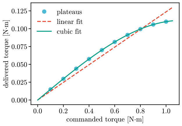
The linear fit gives a constant efficiency of 0.124 (\(R^2\) = 0.949) and misses the bend; the cubic one follows it (\(R^2\) = 1.0000, \(c_3\) = -0.040 against \(-0.04\)).

When one quantity is measured for several motors, such as a fingertip force along a direction, fit_efficiency(commanded, force, weights=w) takes the weights that map each motor’s delivered torque to it. They can come, for example, from the robot’s Jacobian. The finger’s adapt.MOTOR_EFFICIENCY comes from such a fit. With shared=True all motors get one polynomial.