Tuning the damping of a spring¶

In this tutorial we take a fingertip spring of a given stiffness, choose its damping from the finger’s mass, search for the best damping with trial runs, and find the damping beyond which the control loop turns unstable.

The mass the spring moves¶

A spring pulls the fingertip from its start to a goal. The tip responds according to the mass the spring feels along that motion, the effective mass \(m = 1 / (u^\top J M^{-1} J^\top u)\). Here \(M\) is the finger’s mass matrix, \(J\) the tip’s Jacobian and \(u\) the direction of motion:

import numpy as np
import matplotlib.pyplot as plt
import virtualmodelcontrol as vmc
from virtualmodelcontrol import viz
from virtualmodelcontrol.robots import adapt

finger = adapt.add_dynamics(adapt.finger())
kin = vmc.Kinematics(finger)
q0 = np.array([0.3, 0.3])  # [rad], the motors' start
start = kin.position(q0, "tip")
goal = kin.position([0.9, 0.7], "tip")  # [m], a reachable goal

plant = vmc.sim.ModelPlant(finger, q0=q0)
M = np.array(plant.dynamics.mass(q0, plant.p))
J = kin.jacobian(q0, "tip")
u = (goal - start) / np.linalg.norm(goal - start)
m = 1.0 / (u @ J @ np.linalg.solve(M, J.T) @ u)
print(f"effective mass {1000 * m:.1f} g")

effective mass 10.7 g

Stiffness and damping¶

The stiffness \(K\) sets how fast the tip moves, with the natural frequency \(\sqrt{K/m}\), and how hard it holds its goal: a push \(F\) moves it by \(F/K\). The damping \(D\) sets the overshoot: the critical damping \(D_c = 2\sqrt{K m}\) separates a tip that overshoots from one that creeps.

K, dt = 100.0, 1 / 500  # [N/m], and the control period [s]
D_c = 2 * np.sqrt(K * m)

def simulate(D, plant=None, T=1.0):
    ctrl = vmc.Mechanism("ctrl")
    ctrl.add("reach", vmc.LinearSpring(finger.point("tip") - goal, K))
    ctrl.add("damp", vmc.LinearDamper(finger.point("tip"), D))
    ctrl.add("gravity", vmc.GravityCompensation(finger))
    system = vmc.VirtualMechanismSystem(finger, ctrl)
    controller = vmc.VMCController(vmc.compile(system))
    plant = plant or vmc.sim.ModelPlant(finger, q0=q0)
    return vmc.sim.run(plant, controller, vmc.sim.SimClock(dt), T=T)

def distance(log):  # [mm] from the tip to the goal
    tips = np.array([kin.position(q, "tip") for q in log.arrays()["q"]])
    return 1000 * np.linalg.norm(tips - goal, axis=1)

fig, ax = plt.subplots()
for ratio in (0.25, 0.5, 1.0, 2.0):
    log = simulate(ratio * D_c)
    label = f"$D = {ratio:g}\\,D_c$"
    ax.plot(log.arrays()["t"], distance(log), label=label)
ax.set_xlabel("time [s]")
ax.set_ylabel("tip to goal [mm]")
ax.set_xlim(0, 0.5)
ax.legend(fontsize=18);

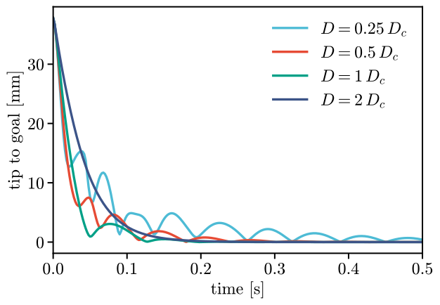
With \(K\) = 100 N/m and a 10.7 g tip, \(D_c\) = 2.07 N·s/m. Below it the tip overshoots the goal and rings. At twice \(D_c\) it arrives later, without overshooting. The formula takes the mass along the motion at the start, and the finger’s mass changes as it moves, so at \(D_c\) itself the tip still goes 1.9 mm beyond the goal.

log = simulate(0.5 * D_c, T=0.4)
viz.animate(finger, log, "tuning.mp4", plane="yz", invert=True,
            springs=[("tip", goal)], trace="tip", speed=0.1)

Search for the damping¶

The damping above came from a formula. A search finds it from runs instead. We write a cost, the distance of the tip to its goal summed over a run, and a searcher picks the dampings to try. Grid, Random, CMAES, ExtremumSeeking and Bayes of vmc.optimization all ask for candidates and are told their costs. The runs in between are yours, in simulation as here or on a robot in your own loop. opt.tune(searcher, cost, rounds) is the loop: rounds times it asks, runs cost on each candidate and tells the costs. The grid gives all its points in its first ask, so one round is enough; Bayes gives its first initial candidates together and then one per ask. A searcher is made from the bounds of the Params: Grid(lower, upper, points), Bayes(lower, upper, initial=...) and Random(lower, upper, size=...). CMAES(start, step, lower, upper, size=...) also takes a starting point and the size of its first steps, and ExtremumSeeking(start, amplitude, gain, ...) the size of its test moves and a gain. The CMA-ES loop below is the same as tune, written out:

from virtualmodelcontrol import optimization as opt


def cost(x):  # [mm s]
    return float(distance(simulate(x[0], T=0.5)).sum() * dt)


grid = opt.tune(opt.Grid([0.1 * D_c], [3 * D_c], 25), cost, rounds=1)

search = opt.CMAES([2 * D_c], 0.5 * D_c, [0.1 * D_c], [3 * D_c], size=6)
for _ in range(5):
    candidates = search.ask()  # the dampings to try
    costs = [cost(x) for x in candidates]  # one run each
    search.tell(candidates, costs)

bayes = opt.tune(opt.Bayes([0.1 * D_c], [3 * D_c], initial=4), cost, 12)

fig, ax = plt.subplots()
x, y = (np.array(h) for h in zip(*grid.history, strict=True))
ax.plot(x[:, 0] / D_c, y, ".-", label="grid")
x, y = (np.array(h) for h in zip(*search.history, strict=True))
ax.plot(x[:, 0] / D_c, y, "o", label="CMA-ES")
x, y = (np.array(h) for h in zip(*bayes.history, strict=True))
ax.plot(x[:, 0] / D_c, y, "s", label="Bayes")
ax.set_xlabel("$D / D_c$")
ax.set_ylabel("cost [mm s]")
ax.legend(loc="upper right", fontsize=18);

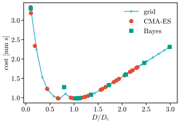
The grid, with 25 runs, puts the best damping at 0.70 \(D_c\), CMA-ES, with 30 runs, at 0.68 \(D_c\), and Bayes, with 12 runs, at 1.04 \(D_c\). The cost is flat near its minimum: the three best costs are within 0.2 % of each other, so the dampings differ more than the costs do. The damping \(D_c\) of the formula costs only 0.4 % more than the best. Bayes fits a Gaussian process to the costs it has seen and asks for the damping where it expects the most improvement, so it suits runs that are few and slow. When the whole motion can be planned, Optimizing a virtual mechanism finds Params with gradients. A search is for when a run is all you have. opt.bounds_of(system.params, names) gives the lower bounds, the upper bounds and the current values of named Params as vectors to start from, and system.params.set_vector(x, names) sets a candidate back.

The loop limits the damping¶

The controller computes the damper’s force from velocities measured at the start of each control period, and a real loop applies it about one period later. A damper that is too strong then overcorrects at every step: the velocity flips sign and grows. For a sampled loop the limit is \(D < 2m/\Delta t\), and with one period of delay \(D < m/\Delta t\).

We find the limits by simulation. The plant below applies each command one step late, like the plant of Extend the library:

class Late:
    """The simulated finger, receiving each command one step late."""

    def __init__(self, plant):
        self.plant, self.u = plant, np.zeros_like(plant.u)

    @property
    def t(self):
        return self.plant.t

    def read(self):
        return self.plant.read()

    def write(self, cmd):
        self.plant.write(vmc.Signals(self.t, motor_torque=self.u))
        self.u = np.array(cmd["motor_torque"], dtype=float)

    def advance(self, dt):
        self.plant.advance(dt)

def unstable(log):  # the tip still moving fast at the end, or diverged
    v = np.diff(distance(log)[-100:]) / dt
    return not np.all(np.isfinite(v)) or np.abs(v).max() > 10.0  # [mm/s]

dampers = np.arange(1.0, 14.0, 0.5)  # [N·s/m]
first = {}
for name, late in (("sampled", False), ("one step late", True)):
    for D in dampers:
        plant = vmc.sim.ModelPlant(finger, q0=q0)
        if unstable(simulate(D, Late(plant) if late else plant)):
            first[name] = float(D)
            break
print(f"m/dt = {m / dt:.1f} N·s/m; first unstable damper: {first}")

m/dt = 5.3 N·s/m; first unstable damper: {'sampled': 12.0, 'one step late': 6.0}

The sampled loop turns unstable at 12.0 N·s/m against \(2m/\Delta t\) = 10.7, and the delayed loop at 6.0 N·s/m against \(m/\Delta t\) = 5.3. Keep the damper well below the limit of your loop. A faster loop, or less delay, allows more damping. A real loop usually has more delay than one step, so its limit is lower.

The runs go unstable above the formulas because the formulas use the mass along the motion at the start. The damper pulls on every direction of the tip, and the lightest one, at the pose where the tip ends, weighs 12.4 g. With that mass the limits are 12.4 and 6.2 N·s/m, which the runs match to within the 0.5 N·s/m of the sweep.

Reading the energies¶

The compiled controller reports its stored energy and the power of its dampers at any state (the energy tutorial lists what energy and power return). Along a run, the spring’s energy should fall as the damper dissipates it:

log = simulate(D_c)
rows = log.arrays()
ctrl = vmc.Mechanism("ctrl")
ctrl.add("reach", vmc.LinearSpring(finger.point("tip") - goal, K))
ctrl.add("damp", vmc.LinearDamper(finger.point("tip"), D_c))
compiled = vmc.compile(vmc.VirtualMechanismSystem(finger, ctrl))
p, z = compiled.live_values(), np.zeros(0)  # no virtual state
V = [float(compiled.energy(q, v, z, p, t)[0])  # the stored energy
     for q, v, t in zip(rows["q"], rows["v"], rows["t"].ravel())]
P = [float(compiled.power(q, v, z, p, t)[1])  # the dampers' power
     for q, v, t in zip(rows["q"], rows["v"], rows["t"].ravel())]
dissipated = -np.cumsum(P) * dt

fig, ax = plt.subplots()
ax.plot(rows["t"], 1000 * np.array(V), label="stored in the spring")
ax.plot(rows["t"], 1000 * dissipated, label="dissipated by the damper")
ax.set_xlabel("time [s]")
ax.set_ylabel("energy [mJ]")
ax.set_xlim(0, 0.5)
ax.legend(fontsize=18);

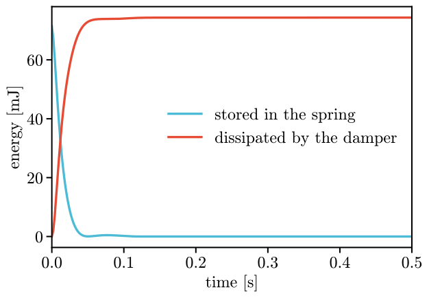
The spring starts with 71 mJ (\(\tfrac12 K d^2\), for the start distance \(d\) to the goal) and has lost 99 % of it after 0.04 s. The damper dissipates 74 mJ, close to that. The difference is the work of the other forces on the finger, gravity and its compensation, which the energy tutorial accounts for.