Energy and passivity¶

In this tutorial we follow the energy of the soft arm and of its controller through a run, check that the energy balance closes, and limit the changes of a running controller with a tank.

Where energy goes¶

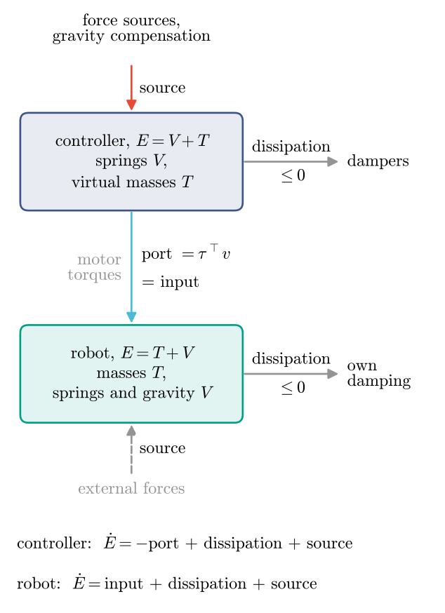
Each mechanism stores energy in its springs and gravity (\(V\)) and in its moving masses (\(T\)). It loses energy in its dampers and receives energy from its sources. The controller and the robot exchange energy only through the motors: the power \(\tau^\top v\) of the controller’s torques leaves the controller as its port and enters the robot as its input. The arrows point the way energy flows when a term is positive. Dissipation is never positive.

The balance in code¶

The compiled controller (law below) and the robot’s dynamics each compute their terms of the figure. ModelPlant compiles the dynamics from the robot mechanism and keeps them as plant.dynamics:

The energies come in opposite orders: (V, T) for the controller, (T, V) for the robot. z holds the controller’s virtual states, its own degrees of freedom (positions, then velocities), p the live Params of each and u the motor torques. The robot’s input equals the controller’s port as long as no output stage (a correction of the commands for real hardware, see Your first controller) changes the torques and the transmission’s efficiency is 1, the default. The soft arm’s tendons really deliver only a share of the motor torque (Transmission efficiency), but its stiffness and damping were identified from the commanded torques, so its model keeps the efficiency 1. To log the controller’s terms during a run, ask vmc.sim.run for record=["energy"] (Run logs).

Check the balance on a run¶

We run the controller of your first controller with a loop faster than on the real arm. The logged steps then resolve the start, where most of the energy changes hands.

import numpy as np
import matplotlib.pyplot as plt
import virtualmodelcontrol as vmc
from virtualmodelcontrol.robots import helyx

arm = helyx.add_dynamics(helyx.arm("145-145-145"))
goal = np.array([0.08, 0.0, 0.40])  # [m]
ctrl = vmc.Mechanism("ctrl")
ctrl.add("reach", vmc.LinearSpring(arm.point(s=1.0) - goal, 300.0))
ctrl.add("damp", vmc.LinearDamper(arm.point(s=1.0), 5.0))
ctrl.add("gravity", vmc.GravityCompensation(arm))
law = vmc.compile(vmc.VirtualMechanismSystem(arm, ctrl))
controller = vmc.VMCController(law)

plant = vmc.sim.ModelPlant(arm)
clock = vmc.sim.SimClock(dt=1 / 5000)  # [s]
log = vmc.sim.run(plant, controller, clock, T=0.2, record=["energy"])
rows = log.arrays()

from virtualmodelcontrol import viz

viz.animate(arm, rows, "energy.mp4", springs=[(1.0, goal)], trace=1.0,
            speed=0.1)

We evaluate the four functions at every logged step. map(n) evaluates a CasADi function on n columns at once.

t = rows["t"].ravel()
q, v = rows["q"].T, rows["v"].T  # a column per step
u = rows["motor_torque"].T
z = np.zeros((0, t.size))  # this controller has no virtual states
p_c, p_r = controller.params, plant.p  # live Params of each


def along(f, *args):
    """f at every step, one array per output."""
    return [x.full().ravel() for x in f.map(t.size)(*args)]


V_c, T_c = along(law.energy, q, v, z, p_c, t)
port, diss_c, src_c = along(law.power, q, v, z, p_c, t)
T_r, V_r = along(plant.dynamics.energy, q, v, p_r, t)
inflow, diss_r, src_r = along(plant.dynamics.power, q, v, u, p_r, t)
float(np.abs(inflow - port).max())  # [W]

3.0828672947791347e-12

At every step the robot receives exactly the power the controller gives. So the energy of the robot plus the energy of the controller changes by what the dampers take and the sources give, integrated over time. What is left over is the residual:

def integral(power):  # from the start to every step [J]
    steps = (power[1:] + power[:-1]) / 2 * np.diff(t)
    return np.concatenate([[0.0], np.cumsum(steps)])


E_c, E_r = V_c + T_c, T_r + V_r
dampers = integral(diss_c + diss_r)
sources = integral(src_c + src_r)
residual = (E_c - E_c[0]) + (E_r - E_r[0]) - dampers - sources

ms = 1000 * t
fig, (top, bottom) = plt.subplots(2, 1, figsize=(6.4, 7.2), sharex=True)
top.plot(ms, E_c - E_c[0], label="controller")
top.plot(ms, E_r - E_r[0], label="robot")
top.plot(ms, dampers, label="dampers")
top.plot(ms, sources, label="sources")
top.set_ylabel("energy [J]")
top.legend(loc="center right", fontsize=18)
bottom.plot(ms, 1000 * residual)
bottom.set_xlabel("time [ms]")
bottom.set_ylabel("residual [mJ]");

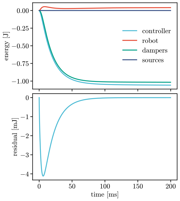
The top panel shows how the energy of each mechanism changed since the start, the energy the dampers took (negative) and the energy the sources gave. The controller’s spring starts with 1.14 J. By 45 ms it has released nine tenths of the energy it releases in this run. Some goes into the arm, whose kinetic energy peaks at 0.05 J, and most into the dampers of the arm and of the controller.

The residual stays within 4.1 mJ, 0.4 % of the energy the dampers took. It is the error of the time steps: the simulator holds each torque for a control period, and we integrate the powers from the logged steps. In this run power flows from the controller to the arm at every step. When an arm swings back against its controller, the port carries energy the other way, and the balance still closes.

The balance from a log¶

A log recorded with record=["energy"] holds the controller’s side of the balance. vmc.sim.energy_balance turns it into the balance of the controller alone: its energy, the work it gave the robot through its port, what its dampers took (dissipated, a positive amount: the dissipation power of the table above is negative) and its sources gave, injected, what is left over, and margin, the energy it can still give, which a passive controller keeps above zero:

b = vmc.sim.energy_balance(log)
for name in ("given", "dissipated", "injected"):
    print(name, round(float(b[name][-1]), 3), "J")

given 0.566 J
dissipated 0.488 J
injected -0.003 J

The controller gave the robot 0.57 J while its dampers took 0.49 J, and injected stays within 4.7 mJ: only the error of the steps. The margin never falls below 0.58 J. A change of a live Param shows up in injected. Here a schedule raises the stiffness to 1500 N/m at 0.1 s, in the middle of the motion:

from virtualmodelcontrol.control import Schedule, ScheduledController

raise_k = Schedule("ctrl.reach.stiffness", [(0.1, 1500.0)], "step")
stiffer = ScheduledController(vmc.VMCController(law), [raise_k])
log2 = vmc.sim.run(vmc.sim.ModelPlant(arm), stiffer, clock, T=0.3,
                   record=["energy"])
b2 = vmc.sim.energy_balance(log2)

fig, ax = plt.subplots()
ax.plot(1000 * b["t"], b["injected"], label="same stiffness")
ax.plot(1000 * b2["t"], b2["injected"], label="stiffer from 0.1 s")
ax.set_xlabel("time [ms]")
ax.set_ylabel("injected energy [J]")
ax.legend(loc="center right", fontsize=18);

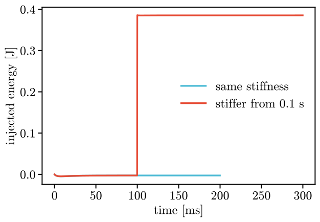
The controller received 0.39 J that no damper or source gave it. A stiffer spring stores more energy at the same deflection, and the energy comes from nowhere. It is the jump that controller.set returns.

Passivity¶

The balance bounds the work that a controller without sources does on the robot:

The bound holds because dissipation is never positive and springs and masses never store negative energy. Whatever the robot does, such a controller can only give back the energy it stored: it is passive. On a robot with only masses, springs, gravity and dampers, the energy of the robot plus the energy of the controller can then only fall.

Gravity compensation is a source, but a tame one. Its forces cancel the weight of the robot’s masses, so the arm moves as if it had no weight. The energy it supplies is only the energy that the robot stores in gravity. This arm is mounted with gravity along \(-y\) and moves in the \(x\)-\(z\) plane, so here it supplies nothing. The controller gave 0.57 J through its port, out of the 1.14 J its spring stored at the start.

Changing a live Param during a run also changes the controller’s energy, by the jump that controller.set returns (Parameters).

Limit changes with a tank¶

Raising a stiffness while the spring is deflected stores energy out of nothing. That breaks the passivity above. A Tank is a budget for such changes to a running controller. It applies a change only as far as the tank can pay for the energy jump: the largest fraction of the step whose exact jump fits. A step that releases energy is always applied whole, and refills the tank:

controller = vmc.VMCController(law)
plant = vmc.sim.ModelPlant(arm)
vmc.sim.run(plant, controller, vmc.sim.SimClock(1 / 330), T=0.05)

tank = vmc.control.Tank(controller, level=0.02)  # [J]
change = {"ctrl.reach.stiffness": 1200.0}
asked = controller.jump(change)  # the whole step [J]
paid = tank.set(change)
fraction = tank.fraction
print(f"asked {asked:.3f} J, paid {paid:.3f} J: {fraction:.2f} of the step")
freed = -tank.set({"ctrl.reach.stiffness": 100.0})
print(f"released {freed:.3f} J, the tank holds {tank.level:.3f} J")

asked 0.537 J, paid 0.020 J: 0.04 of the step
released 0.139 J, the tank holds 0.139 J

controller.jump(values) is the jump controller.set(values) would give, without applying it. The tank is otherwise the controller: run it in place of the controller. Pass a result of an optimization to result.apply(tank), so that an optimizer’s new gains reach the robot only as fast as the budget allows.

The tank fills itself in a run. Run in place of the controller, it takes in at every step what the controller’s own dampers took:

tank = vmc.control.Tank(vmc.VMCController(law))  # empty
vmc.sim.run(vmc.sim.ModelPlant(arm), tank, clock, T=0.2)
print(f"{tank.level:.3f} J")

0.488 J

The level is 0.49 J, the energy the dampers took in the balance above. A change that raises the controller’s energy can now be paid from it.

A stiffness that a law proposes¶

A stiffness that a law proposes can be indefinite or not symmetric, and then a spring with it can store negative energy. project_psd gives the nearest symmetric positive semidefinite matrix. Pass a proposed stiffness through it before it reaches set or a tank:

K = np.array([[300.0, 450.0], [0.0, 100.0]])
vmc.control.project_psd(K).round(1)

array([[313.7, 203.9],
       [203.9, 132.5]])

Where to go next¶

Tuning the damping of a spring uses these energies to find the damping that a sampled loop can bear, and Robots with fewer motors than joints keeps a controller passive when some joints have no motor. The equations behind the balance are in Passivity.