Passivity¶

A controller built from springs and dampers can only give the robot back the energy it stored. This page states that property, shows how it makes the robot and its controller stable together, and lists what weakens it in practice. Energy and passivity checks the same balance numerically on a run.

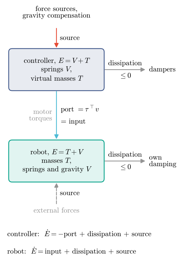
The controller’s energy balance¶

The controller stores \(E_c = V + T\): \(V\) in its springs, measured from its lowest value so that \(E_c \ge 0\), and \(T\) in the inertances of its virtual states. Three powers change it. The port, \(P = \tau^\top v\), is the power its torques give the robot. The dissipation power is \(P_D = \sum f \cdot \dot y \le 0\) over its dampers. The source power is \(P_S = \sum f \cdot \dot y\) over its sources. With the VMC equations,

The compiled controller computes each term (compiled.energy, compiled.power), so the balance can be checked on any run.

Passive controllers¶

Without sources, integrating the balance gives

since \(E_c(t) \ge 0\) and \(P_D \le 0\). Whatever the robot does, the controller gives it at most the energy it stored at the start: it is passive.

The robot and its controller together¶

A robot made of masses, springs, dampers and gravity is passive too: its energy \(E_r\) changes by its input power and its own dissipation. With the default efficiency of 1 and no output stage, its input power is the controller’s port \(P\), so the two balances add up:

Without sources the total energy can only fall. It is bounded by its value at the start. Where it has a minimum, at the equilibrium the springs set, it works as a Lyapunov function: the robot settles there or stays near it.

Gravity compensation is a source, but its forces are exactly those that cancel the weight of the robot’s masses: its power is minus the power of gravity on them. Added to the balance, it removes gravity’s potential energy from the robot’s. The robot then behaves as if it had no weight.

What weakens it¶

• Sampling and delay. A digital controller holds each torque for a control period, so it reacts to the past. Stiff springs and strong dampers then inject energy. Above a point the loop goes unstable even though every element is passive. Tuning shows the limit on damping.

• Changing parameters while running. Raising a stiffness raises the energy stored in that spring at once; controller.set returns that jump (Parameters), and a Tank pays for it (Energy and passivity). Swapping elements through a smooth blend (vmc.control.SwapController) keeps the torques continuous.

• Sources. A force source can supply any energy; only gravity compensation is tame.

• Efficiency. One constant efficiency \(\eta\) on every motor scales the robot’s input to \(\eta P\), and the balance holds with \(\eta E_c\). Different efficiencies on motors that one element couples make its forces non-conservative, as the finger example explains.

• Joints that no motor drives. Torques that the motors alone can give, \(B^+\tau\), are not the gradient of a potential, so the controller may not be passive any more. Robots with fewer motors than joints shows the controllers that keep it passive.

• Output stages. Friction compensation, pretension and torque limits change the torques the motors receive, so the robot’s input is no longer the controller’s port.