Static friction of the motors¶

A motor does not deliver a small torque: friction holds it until the command passes a breakaway value. A virtual spring that pulls with less than that does not move the joint, and the robot stops short of its goal. In this tutorial we model that friction as a function of the torque we apply, see what it does to a controller, compensate it, identify it from data, and plan with it. Everything here is off unless we ask for it.

The model¶

StaticFriction(breakaway, kinetic, width) is the torque \(\tau_f\) that friction takes from a motor, as a function of the torque \(u\) we apply to it, in N·m. Below the breakaway torque \(F\) the motor is stuck: friction takes all of \(u\). Past it the motor moves, and friction takes the kinetic torque \(F_c\), with the sign of \(u\). With \(F_c = 0\) the static friction is gone once the motor moves, and with \(F_c = F\) it stays. Around \(|u| = F\) the change is smooth over width, and the whole map is smooth, so a solver can differentiate it. It depends on the torque only, not on the speed.

import numpy as np
import matplotlib.pyplot as plt
import virtualmodelcontrol as vmc

F = 0.2  # breakaway torque [N·m]
u = np.linspace(-0.6, 0.6, 601)  # commanded torque [N·m]

fig, (top, bottom) = plt.subplots(2, 1, sharex=True)
for Fc, style in ((0.0, "-"), (F, "--")):
    friction = vmc.StaticFriction(F, Fc, 0.01)
    top.plot(u, friction(u), style, label=f"$F_c$ = {Fc}")
    bottom.plot(u, u - friction(u), style)
top.set_ylabel(r"friction $\tau_f$")
top.set_ylim(-0.3, 0.6)  # room for the legend
bottom.set_ylabel(r"delivered $u - \tau_f$")
bottom.set_xlabel(r"commanded torque $u$ [N$\cdot$m]")
top.legend(loc="upper left", fontsize=18);

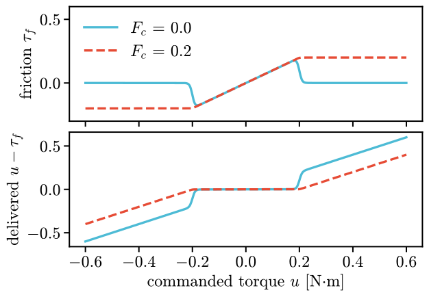
The motor delivers nothing in the dead band, and then the command less \(F_c\). The default is \(F = F_c = 0\), which is no friction at all. The three numbers are Params of scope design (Parameters), to tune or to identify.

In a robot¶

Friction belongs to the motor, so it goes with the robot’s transmission: its Efficiency takes a friction. An Efficiency(c) makes the robot receive \(c\,u\) for the torque \(u\) commanded (Efficiency), and Efficiency(1.0), the default, loses nothing. Here is a joint with an inertia and a damper, and a virtual spring of 1 N·m/rad that pulls it to 1 rad:

from virtualmodelcontrol.models import Direct, Efficiency, JointSpace

def system_of(friction=None, stiffness=1.0):
    efficiency = Efficiency(1.0, friction=friction)
    robot = vmc.Mechanism("robot", model=JointSpace(1, unit="rad"),
                          actuation=Direct(efficiency))
    q = robot.joint(0)
    robot.add("inertia", vmc.Inertance(q, 1.0))  # [kg·m²]
    robot.add("damper", vmc.LinearDamper(q, 1.5))  # [N·m·s/rad]
    ctrl = vmc.Mechanism("ctrl")
    goal = vmc.Ref("goal", 1, [1.0])  # [rad]
    ctrl.add("spring", vmc.LinearSpring(q - goal, stiffness))
    ctrl.add("damper", vmc.LinearDamper(q, 1.0))
    return vmc.VirtualMechanismSystem(robot, ctrl)

def run(system, output=(), T=30.0):
    plant = vmc.sim.ModelPlant(system.robot)
    controller = vmc.VMCController(vmc.compile(system), output=list(output))
    clock = vmc.sim.SimClock(dt=1 / 100)
    return vmc.sim.run(plant, controller, clock, T=T).arrays()

We run it without friction, and with friction that stays at 0.3 N·m once the motor moves:

kept = vmc.StaticFriction(0.3, 0.3, 0.005)
free, held = run(system_of()), run(system_of(kept))

fig, ax = plt.subplots()
ax.plot(free["t"], free["q"][:, 0], label="no friction")
ax.plot(held["t"], held["q"][:, 0], "--", label=r"friction 0.3 N$\cdot$m")
ax.set_xlabel("time [s]")
ax.set_ylabel("angle [rad]")
ax.legend(loc="lower right", fontsize=18);

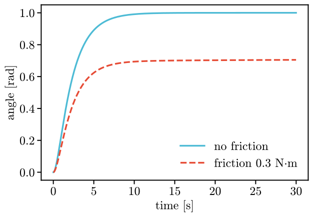
The joint without friction arrives. With it, the joint stops 0.30 rad short: the spring pulls with \(K e\), and the motor is stuck while that is below the breakaway torque, so it stops at \(e = F / K\). A stiffer spring narrows the gap, and a spring that is too soft for the friction does not move the joint at all.

Compensation¶

The compensation adds the friction to the command, in the direction of the command: \(u + F_c u / \sqrt{u^2 + w^2}\), smooth in \(u\), with \(w\) the width. StaticFrictionCompensation.of(friction) takes \(F_c\) and the width from a StaticFriction, and an optional fraction of it. It is an output stage: a correction that VMCController(output=...) applies to the command after the controller’s law (the loop). Nothing turns it on but us:

from virtualmodelcontrol.control import StaticFrictionCompensation

full = StaticFrictionCompensation.of(kept)
half = StaticFrictionCompensation.of(kept, fraction=0.5)
stages = {"none": [], "half": [half], "full": [full]}
errors = {name: 1.0 - run(system_of(kept), stage)["q"][-1, 0]
          for name, stage in stages.items()}
errors

{'none': np.float64(0.29514864882423686),
 'half': np.float64(0.14531043407002253),
 'full': np.float64(0.010633867285968823)}

Compensating all of the friction leaves 0.011 rad, and half of it leaves 0.15 rad. The compensation is exact only for the kinetic torque: if the breakaway torque \(F\) is larger than \(F_c\), a band of \(F - F_c\) is left, because a command that is not enough to break away is not enough with the compensation either.

The compensation adds energy: it pushes with \(F_c\) in the direction of the command, which is up to \(F_c |\dot\theta|\) of power. The friction map has its own limit. It depends on the torque alone, so it does not know which way the motor moves. When a command brakes the motion, the map takes from the braking torque and can create power, up to \(F |\dot\theta|\):

friction = vmc.StaticFriction(F, 0.0, 0.01)
rate = np.linspace(-3, 3, 61)  # [rad/s]
power = friction(u)[:, None] * rate[None, :]  # friction torque times rate
created = -power.min()  # [W]
created, F * abs(rate).max()

(np.float64(0.5270943881766896), np.float64(0.6000000000000001))

So the friction is dissipative when the command and the motion agree, and otherwise creates at most 0.53 W here, at 3 rad/s, under the bound \(F |\dot\theta|\) of 0.6 W. A passivity argument that counts on the motors’ friction can count on no more than that.

Identification¶

The three numbers are Params of the robot, so fit_params finds them from a run, with the stiffness and damping, as Fit Params to a run shows. Their names say where they sit: efficiency.friction.breakaway is the breakaway of the friction of the robot’s efficiency (robot.params lists all of them). The command has to rise slowly from rest, a ramp, or the breakaway torque does not show: after a step the motor has broken away at the first sample. We simulate a robot with friction under a ramp of torque, up and down, and fit from a rough guess:

from virtualmodelcontrol.identification import fit_params

dt = 1 / 330
rise = np.arange(0.0, 0.8, 0.5 * dt)  # [N·m], 0.5 N·m/s
command = np.concatenate([np.zeros(150), rise, rise[::-1], np.zeros(150)])

truth = vmc.StaticFriction(0.3, 0.1, 0.002)
robot = system_of(truth).robot
robot.add("spring", vmc.LinearSpring(robot.joint(0), 40.0))
# no controller:
bare = vmc.VirtualMechanismSystem(robot, vmc.Mechanism("none"))
log = vmc.sim.rollout(bare, [0.0], len(command) * dt, dt, max_step=dt,
                      u=command[:, None])

guess = system_of(vmc.StaticFriction(0.2, 0.05, 0.002)).robot
guess.add("spring", vmc.LinearSpring(guess.joint(0), 30.0))
names = ["efficiency.friction.breakaway", "efficiency.friction.kinetic",
         "spring.stiffness"]
fit = fit_params(guess, names, [log], smoothing=11)
for name in names:
    print(name, fit.values[name].ravel().round(3))

efficiency.friction.breakaway [0.3]
efficiency.friction.kinetic [0.102]
spring.stiffness [39.881]

The fit gives 0.30 N·m for the breakaway and 0.10 N·m for the kinetic torque, against 0.30 and 0.10 in the simulated robot. The fit is local: it starts from the robot’s values, and a start far from the truth can end in a wrong one, so the first command at which the motor moved is a good guess for the breakaway torque. If we have the delivered torque of each motor at static commands, from a load cell, fit_efficiency(commanded, delivered, friction=True) fits the efficiency and the friction together; the points must cover the dead band, on both sides.

from virtualmodelcontrol.identification import fit_efficiency

commanded = np.linspace(-1.0, 1.0, 81)[:, None] * np.ones((1, 2))  # [N·m]
dead = vmc.StaticFriction([0.25, 0.15], 0.05)  # breakaway of each motor
motors = Efficiency((0.8, 0.6), friction=dead)
efficiency = fit_efficiency(commanded, motors(commanded), friction=True,
                            width=0.01)
efficiency.friction.params["breakaway"].value.round(2)

array([0.25, 0.15])

Planning with it¶

The friction is in the robot’s dynamics, so a plan (Optimize), an optimization and an MPC (Model predictive control) see it. A compensation joins them through Problem(output=...), which applies the stage to the controller’s command as VMCController(output=...) does in a simulation:

from virtualmodelcontrol import optimization as opt

smooth = vmc.StaticFriction(0.3, 0.3, 0.02)  # wider: easier for a solver
stage = StaticFrictionCompensation.of(smooth, fraction=0.7)
system = system_of(smooth)

problem = opt.Problem(system, output=[stage])
problem.add(opt.Shooting([0.0], 3.0, 11, v0=[0.0], substeps=5))
plan = problem.solve()
sim = vmc.sim.rollout(system, [0.0], 3.0, 0.06, v0=[0.0], max_step=0.06,
                      output=[stage])
gap = abs(plan.q[:-1] - sim["q"][::5]).max()

The plan follows the simulation within 2e-11 rad: it is the same closed loop, with the motor’s friction and the compensation in it. The plan has a point every 0.3 s, which is every fifth step of the simulation. MPC(problem) takes the same problem, so it plans with friction too.

Good to know¶

• Off by default. Efficiency(friction=None) and StaticFriction() with no torques are the robots as they were, and no template turns the compensation on. The finger’s and the hand’s values, adapt.finger_friction() and adapt.hand_friction(), are there to ask for.

• The width is the smoothing of the corner at the breakaway torque, in N·m. A smaller one is closer to a real motor and harder for a solver: a plan from rest may need a warm start.

• No memory. The map depends on the torque we apply and not on how the motor got there, so it has no hysteresis: a real motor that has stopped holds up to \(F\) against the net torque, load included.

• Where it acts. The friction takes its torque from the command before the efficiency polynomial, in the units of the command.