Virtual Model Control¶

Virtual Model Control (VMC) builds a controller from virtual mechanical elements attached to the robot. This page gives the equations behind it: coordinates, the forces of the elements, the motor torques that realize them, and the controller’s own degrees of freedom. How it works introduces the idea without the mathematics.

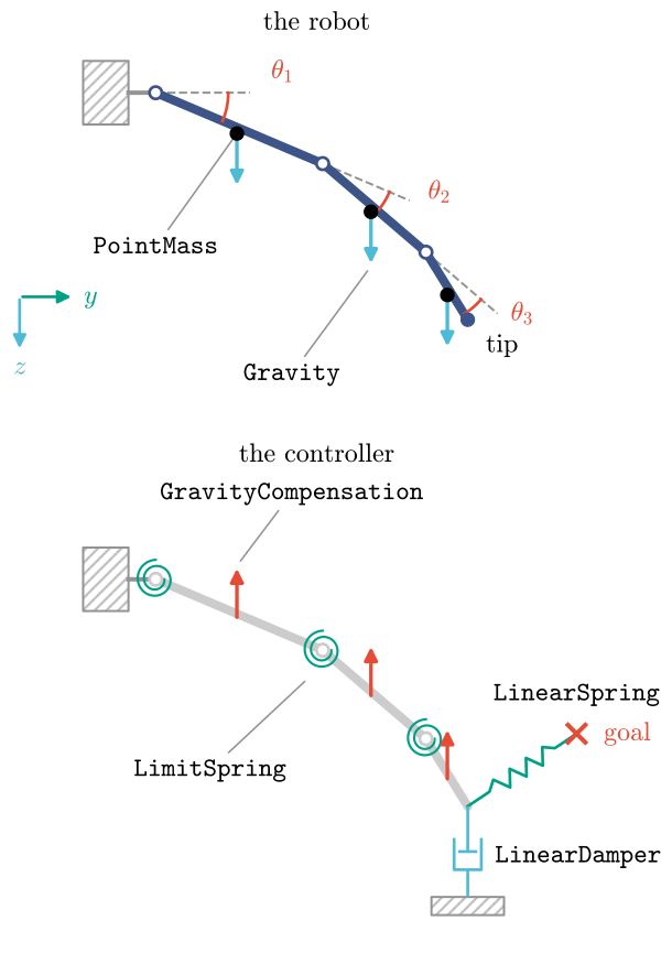
../_images/ce8457dc326fa58ec6465a8c189d7f2ac91f84799743571d5f7bf127d1d043fe.svg

Coordinates¶

A virtual element acts on a coordinate, a function of the robot’s configuration \(q\), of the controller’s virtual states \(z\) and of time:

\[ y = h(q, z, t), \]

such as a point of the body minus a goal, the projection of that difference on a direction, or a distance to a surface. Its rate follows by the chain rule,

\[ \dot y = J_q\,v + J_z\,\dot z + \frac{\partial h}{\partial t}, \qquad J_q = \frac{\partial h}{\partial q}\,G(q),\quad J_z = \frac{\partial h}{\partial z}, \]

with \(v\) the robot’s velocity and \(G\) the map from velocities to configuration rates (the identity for most robots). The library differentiates every coordinate exactly, so \(J_q\) and \(J_z\) need no hand derivation.

Elements and their forces¶

Each element gives a force \(f\) on its coordinate. Springs store energy, \(f = -\partial V/\partial y\) with \(V\) bounded below. A linear spring of stiffness \(K\) on \(y = x - x_\text{ref}\) pulls \(x\) towards \(x_\text{ref}\) with \(f = -K y\). Dampers dissipate, \(f \cdot \dot y \le 0\), as \(f = -D \dot y\). Inertances give mass to a virtual state of the controller, or to a coordinate of the robot. Sources add forces of their own, such as gravity compensation, \(f = -m g\) on each of the robot’s masses \(m\), with \(g\) the gravity vector.

From forces to motor torques¶

The torque that a force \(f\) on \(y\) exerts on the robot follows from power: \(f \cdot \dot y = \tau^\top v\) for every velocity \(v\), so

\[ \tau = \sum_k J_{q,k}^\top f_k , \]

the sum over the controller’s elements. The motors then deliver it: their torques \(u\) solve

\[ B(q)\,u = \tau , \]

with \(B\) the robot’s actuation map. For a tendon arm \(B = (\partial\theta/\partial q)^\top\), with \(\theta\) the motor angles. With one motor per joint \(B\) is the identity. The controller never divides \(u\) by an efficiency. A robot with fewer motors than joints has no \(u\) that solves it for every \(\tau\): the motors give the least-squares \(u = B^+\tau\), and the part of \(\tau\) outside the range of \(B\), which they cannot give, is the torque defect of the underactuated tutorial.

Virtual states¶

A controller may have degrees of freedom of its own, \(z\), with virtual inertances \(M_z\). The same forces drive them,

\[ M_z\,\ddot z = \sum_k J_{z,k}^\top f_k - c(z, \dot z), \]

with \(c\) the velocity terms of \(M_z\). The controller integrates them at every step. A virtual flywheel that the turtle’s cranks follow is such a state (turtle example).

The compiled controller¶

vmc.compile writes all of this as one CasADi function. Its inputs are the motor angles and rates, the virtual states and the live parameters. Its outputs are the motor torques and the virtual states’ rates. The robot’s configuration follows from the motor angles through the exact inverse of its transmission. The controller’s energy and power, used on Passivity, come from the same graph.