Crawl with a flywheel¶

In this tutorial a crawler crawls across the ground in simulation. Two cranks push it forward, one per side, and one virtual flywheel keeps them in step. We see how a virtual state drives a gait, shape the stiffness of the springs with the flywheel’s phase, steer, let the crawler find its own gait by search, and plan a stride with the optimizer.

One flywheel, two cranks¶

A rhythmic gait needs its cranks to turn together, a fixed phase apart. The usual controller gives each crank a clock and a reference to follow. A moving reference puts energy into the loop that nothing accounts for, and two clocks drift apart. Here the clock is a physical object: one virtual flywheel, with an inertia and a constant drive, tied to each crank by a spring. The phase offset between the sides is a constant, so the gait phase is exact. The flywheel stores what the springs give it, so the loop is passive. If a foot catches, its spring stretches and slows the flywheel, and the other crank slows with it.

The flywheel has an angle \(\varphi\). Side \(i\) runs at the phase \(\varphi_i = \varphi - \Delta_i\), and its spring is stretched by \(e_i = q_i - \varphi_i\), with \(q_i\) the crank angle. The stiffness follows the phase, and the torque on the crank is

\(\bar K\) is the mean stiffness, \(C\) the damping of each spring. The depth \(m\) (between 0 and 0.9) and the peak \(\varphi_K\) shape the stiffness, and the steering \(u_s\) makes one side stiffer and the other softer. The flywheel has the inertia \(J_v\), and \(b_v\) is both the friction it feels and the gain of its drive \(b_v\bar\omega\). With \(K_i' = \mathrm{d}K_i/\mathrm{d}\varphi\) it obeys

The term \(-\tfrac12 K_i' e_i^2\) is the reaction of a stiffness that changes with the phase: stiffening a stretched spring costs energy, and the flywheel pays it. PhaseSpring is the spring whose energy depends on both the stretch and the phase, so its force on the phase is exactly this term.

The controller¶

The crank angles are the robot of the controller: turtle.robot() holds only \(q\) = (left, right) [rad]. The controller adds the flywheel as a virtual state with an inertia, a speed regulator for the drive, and for each side a PhaseSpring on the pair (stretch, phase) and a damper on the stretch. The right side runs \(\Delta\) behind the left one. With \(\Delta = \pi\) the cranks are half a turn apart, a diagonal gait.

import numpy as np
import matplotlib.pyplot as plt
import virtualmodelcontrol as vmc
from virtualmodelcontrol import viz
from virtualmodelcontrol.robots import turtle

robot = turtle.robot()  # the two cranks
bv = 0.3  # b_v: the flywheel's friction and its drive's gain [N·m·s/rad]

def flywheel(omega, depth=0.0, steer=0.0, peak=0.0, delta=np.pi):
    ctrl = vmc.Mechanism("ctrl")
    phi = ctrl.add_state("flywheel", unit="rad")
    ctrl.add("flywheel", vmc.Inertance(phi, 0.24))  # J_v [kg·m²]
    ctrl.add("drive", vmc.SpeedRegulator(phi, bv, omega, 0.5))
    behind = vmc.Ref("delta", 1, value=delta, unit="rad")
    for i, (phase, side) in enumerate([(phi, 1.0), (phi - behind, -1.0)]):
        e = robot.joint(i) - phase  # the stretch of the spring
        spring = vmc.PhaseSpring(vmc.Stack(e, phase), 1.0, depth=depth,
                                 peak=peak, steer=steer, side=side)
        ctrl.add(f"spring{i}", spring)  # K [N·m/rad]
        ctrl.add(f"damper{i}", vmc.LinearDamper(e, 0.06))  # C
    return ctrl

omega is the speed \(\bar\omega\) [rad/s] the flywheel is driven to, reached over a ramp of 0.5 s. side is \(\pm1\) in \((1 \pm u_s)\): the left spring is stiffer than the right one for a positive steer. The controller does not know the body: it turns the two crank angles it measures into two torques. We call it once at rest, with no simulation:

system = vmc.VirtualMechanismSystem(robot, flywheel(omega=6.0, depth=0.5))
controller = vmc.VMCController(vmc.compile(system))
meas = vmc.Signals(0.0, motor_position=[0.0, -np.pi],
                   motor_velocity=[0.0, 0.0])
controller.reset(0.0, meas, z0=turtle.initial_state(meas))
torque = controller.step(0.01, meas)["motor_torque"]
float(abs(torque).max())  # [N·m]

0.0

The cranks sit where the springs want them, so the torques are zero. Nothing else is needed on the real robot: controller.step(t, measurements) returns the motor torques.

The crawler¶

To see the controller work we need a body. turtle.crawler() is a simple crawler for the simulator: a floating body that lies on the ground \(z = 0\) with gravity, and two cranks that turn about its lateral axis, each with a foot 5 cm from the axis. At each foot and at the four corners of the underside, a contact spring, a contact damper and friction hold the body up. The cranks are the only motors; the body has none. It is a stand-in with placeholder constants (turtle.CRAWLER); its numbers are not measured.

The simulator runs the crawler, and the controller still sees only the two cranks. This is the split of the table in the contact tutorial: the world belongs to the simulated robot, not to the controller. The crawler’s \(q\) holds the body’s position and quaternion \((x, y, z, q_w, q_x, q_y, q_z)\), then the two cranks. We start the body 4 cm above the ground, level and facing \(+x\), with the left foot down and the right one up:

def crawl(omega=6.0, depth=0.0, steer=0.0, peak=0.0, T=8.0, **body):
    ctrl = flywheel(omega, depth, steer, peak)
    system = vmc.VirtualMechanismSystem(robot, ctrl)
    controller = vmc.VMCController(vmc.compile(system))
    q0 = [0, 0, 0.04, 1, 0, 0, 0, 0.0, -np.pi]  # x y z, quaternion, cranks
    plant = vmc.sim.ModelPlant(turtle.crawler(**body), q0=q0, max_step=1e-3)
    clock = vmc.sim.SimClock(1 / turtle.CONTROL_RATE)
    return vmc.sim.run(plant, controller, clock, T=T,
                       z0=turtle.initial_state, record=["energy"])

log = crawl()
rows = log.arrays()
t, q = rows["t"].ravel(), rows["q"]

max_step=1e-3 is a step small enough to follow the contacts. We read the position of the body and the crank angles from the log.

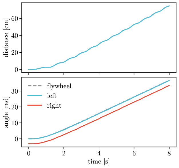
The body moved 0.75 m forward in eight seconds. The top panel shows its distance and the bottom one the crank angles. The cranks run half a turn apart from the start, and the left one follows the flywheel. The body does not go at a constant speed: at its fastest it moves 1.8 times as fast as its mean.

The flywheel under load¶

The flywheel is driven to \(\bar\omega\) = 6 rad/s, and the cranks load it, so it runs slower. Over whole turns, \(b_v(\bar\omega - \langle\dot\varphi\rangle)\) is the mean torque the cranks take from the springs. The slowdown measures the load, and a constant drive needs no sensor for it.

omega = 6.0  # the commanded speed [rad/s]
phi, torque = rows["z"][:, 0], rows["motor_torque"]
turns = np.floor(phi / (2 * np.pi)).astype(int)
first, last = (int(np.argmax(turns >= n)) for n in (2, turns.max()))
speed = (phi[last] - phi[first]) / (t[last] - t[first])  # [rad/s]
load = torque[first:last].sum(axis=1).mean()  # [N·m]
print(f"speed {speed:.2f} rad/s, b_v (omega - speed) = "
      f"{bv * (omega - speed):.3f} N·m, mean torque {load:.3f} N·m")

speed 5.19 rad/s, b_v (omega - speed) = 0.243 N·m, mean torque 0.239 N·m

The flywheel runs 13% below its commanded speed, at 5.19 rad/s. The two torques printed above agree to 2%.

The shape of the stiffness¶

depth is \(m\), how much the stiffness swings over a turn. At 0 the spring is a plain one. At 0.9 it is 19 times stiffer at its peak than a half turn later. peak is \(\varphi_K\), the phase of the stiffest moment. The left crank has its foot at the bottom at the phase 0, so peak=0 is a stiff spring while the foot pushes and a soft one while it swings. We crawl at the depth 0.9 with eight peaks, and compare with the plain spring.

peaks = np.linspace(0, 2 * np.pi, 8, endpoint=False)
logs = {a: crawl(depth=0.9, peak=a) for a in peaks}
reach = np.array([100 * log.arrays()["q"][-1, 0] for log in logs.values()])
plain = 100 * q[-1, 0]  # [cm], the plain spring of the first run

fig, ax = plt.subplots()
ax.axhline(plain, color=viz.PALETTE[9], ls="--", label="plain spring")
ax.plot(peaks, reach, "o-", label="$m$ = 0.9")
ax.set_xlabel(r"peak phase $\varphi_K$ [rad]")
ax.set_ylabel("distance in 8 s [cm]")
ax.legend();

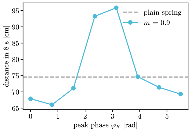
The plain spring takes the body 75 cm. A stiff spring in stance (peak=0) takes it 68 cm, and the opposite (peak = \(\pi\), soft in stance) 96 cm, 29% further than the plain one. This depends on the body, so on yours the best peak may be elsewhere. What does not depend on it is passivity: every run keeps the controller’s energy balance above zero (see Energy and passivity), because the flywheel pays for the changes of stiffness.

Steering¶

steer is \(u_s\): the left spring has the stiffness \((1 + u_s)\) and the right one \((1 - u_s)\) times the mean. The two sides then push unequally and the body turns. We crawl twelve seconds with a steer of \(-0.8\), 0 and \(0.8\), and draw the path seen from above.

paths = {u: crawl(depth=0.5, steer=u, T=12.0) for u in (-0.8, 0.0, 0.8)}

fig, ax = plt.subplots(figsize=(6.4, 4.4))
for u, log in paths.items():
    q_u = log.arrays()["q"]
    ax.plot(100 * q_u[:, 0], 100 * q_u[:, 1], label=f"$u_s$ = {u}")
ax.set_aspect("equal")
ax.set_xlabel("forward [cm]")
ax.set_ylabel("left [cm]")
ax.legend();

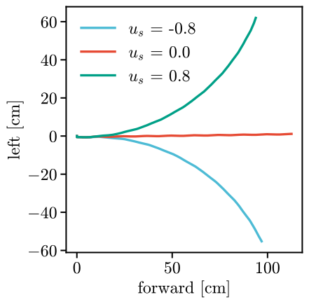
A positive steer turns this crawler to the left, a negative one to the right, by the same amount: 0.14 rad per turn of the flywheel at \(|u_s|\) = 0.8. The turning depends on the body: on another robot the stiffer side may push more or less, so check the sign on yours. The gait phase does not break, because both sides still ride the same flywheel: steering changes only how hard each side pushes. Keep \(|u_s|\) below 1, or one spring loses all its stiffness.

Let the crawler find its gait¶

The best peak depends on the body, and we do not know the body. DitherSeeking finds it from the gait’s own result. It holds the Param at an estimate plus a slow sinusoidal dither, measures how the cost, here minus the forward speed, follows the dither, and moves the estimate downhill. The tone must be slow against the gait: its period is the window, six seconds against strides of a second, and frequency is \(2\pi n/\)window for a whole \(n\), so that several Params, each with its own \(n\), do not see one another. amplitude is the dither’s size [rad], and gain turns the slope of the cost into the estimate’s rate of change. Every change goes through a Tank, whose energy comes from what the controller’s dampers take: a change that would cost more than the tank holds is cut short. This is the passivity bound on a slow change of a potential (Passivity). One Param is shared by the two springs, so that they move together:

from virtualmodelcontrol.adaptation import DitherSeeking
from virtualmodelcontrol.control import Tank

peak = vmc.Param("peak", 0.0, unit="rad", scope="stage",
                 bounds=(-np.inf, np.inf))  # one Param, both springs
system = vmc.VirtualMechanismSystem(robot, flywheel(6.0, 0.9, peak=peak))
tank = Tank(vmc.VMCController(vmc.compile(system)), capacity=1.0)
window = 6.0  # [s]
law = DitherSeeking(tank, "ctrl.spring0.peak", amplitude=0.8,
                    frequency=2 * np.pi / window, gain=12.0, window=window)
plant = vmc.sim.ModelPlant(turtle.crawler(), max_step=1e-3,
                           q0=[0, 0, 0.04, 1, 0, 0, 0, 0.0, -np.pi])
tank.reset(0.0, plant.read(), z0=turtle.initial_state(plant.read()))
dt = 1 / turtle.CONTROL_RATE
seen = []
for step in range(int(120 / dt)):
    plant.write(tank.step(plant.t, plant.read()))
    law.step(tank, -plant.v[0], plant.t)  # the cost: minus the speed [m/s]
    if step % 45 == 0:
        seen.append((plant.t, plant.v[0], law.estimate[0], tank.level))
    plant.advance(dt)
seen = np.array(seen)

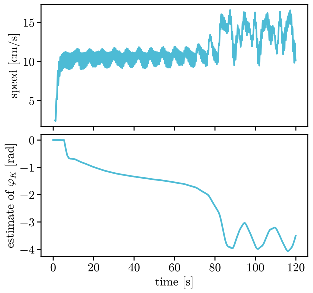
The crawler starts at 9.4 cm/s with the stiff-in-stance spring and, in two minutes of simulated time, learns to go at 13.7 cm/s, 46% faster. Its estimate of peak ends at 2.8 rad (modulo a turn), within 0.4 rad of the \(\pi\) of the sweep above. The tank started empty, filled from what the dampers took, and never went below zero. On a real robot the cost is a measured speed, or a cost of transport from the flywheel’s speed, and the run is a long one that you leave alone.

Plan the crawler¶

The planner can run the flywheel controller on the crawler too. Problem(system, plant=body) takes the dynamics from body, the crawler, while the controller stays the one written for the two cranks: it reads the motors of the plant as it does in a simulation. We plan 0.8 s of the gait, 120 steps at 150 Hz (a third of the crawler’s control rate), from a flywheel that is up to speed (no ramp), once with the stiffness peak at 0. A Shooting is the closed loop of the simulator, step for step, so we start it from the simulated run, which it must reproduce:

from virtualmodelcontrol import optimization as opt

peak = vmc.Param("peak", 0.0, unit="rad", scope="stage",
                 bounds=(-np.pi, np.pi))
gait = flywheel(6.0, 0.9, peak=peak)
gait.params["drive.ramp_time"].value = 0.0  # the flywheel starts at speed
body = turtle.crawler()
dt, n = 1 / 150, 120  # a control step [s], and the steps of the plan
q0 = [0, 0, 0.04, 1, 0, 0, 0, 0.0, -np.pi]
start = [0.0, 6.0]  # the flywheel's angle [rad] and speed [rad/s]

def simulate(angle):
    peak.value = angle
    system = vmc.VirtualMechanismSystem(robot, gait)
    plant = vmc.sim.ModelPlant(body, q0=q0, max_step=dt)
    controller = vmc.VMCController(vmc.compile(system))
    return vmc.sim.run(plant, controller, vmc.sim.SimClock(dt),
                       T=(n + 1) * dt, z0=lambda meas: np.array(start)
                       ).arrays()

run = simulate(0.0)
system = vmc.VirtualMechanismSystem(robot, gait)
problem = opt.Problem(system, plant=body)
problem.add(opt.Shooting(q0, n * dt, n + 1, v0=np.zeros(8), z0=start,
                         running=False))
guess = {"q": run["q"][: n + 1], "v": run["v"][: n + 1],
         "z": np.vstack([start, run["z"][:n]])}  # z is logged after a step
plan = problem.solve(warm_start=guess)
print(plan.status, plan.iterations, plan.violation)

Solve_Succeeded 0 2.495781359357352e-13

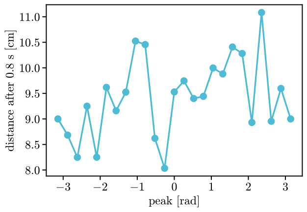
The plan has no work to do: the simulated run satisfies the program’s equations to rounding error (9.5 cm in 0.8 s), so the planner and the simulator are the same loop, with the contact, the friction and the flywheel’s own motion. To search for a gait with it we free the peak and ask the body to go as far as it can. The distance after the 0.8 s, as a function of the peak, shows what the search is up against:

angles = np.linspace(-np.pi, np.pi, 25)
reach = np.array([simulate(a)["q"][n, 0] for a in angles])  # [m]
fig, ax = plt.subplots()
ax.plot(angles, 100 * reach, "o-")
ax.set_xlabel(r"peak [rad]")
ax.set_ylabel("distance after 0.8 s [cm]");

Now we free the peak and ask for the body to be as near as it can to a point 1 m ahead at the end of the plan, which is as far as it can get. The planner starts from the peak at 0:

peak.value = 0.0
problem.add(opt.Cost(body.joint(0) - 1.0, 1.0, t_from=(n - 1) * dt,
                     name="forward"))
problem.free("ctrl.spring0.peak")
planned = problem.solve(warm_start=guess)
planned.params["ctrl.spring0.peak"]

array(0.00087555)

The distance after the 0.8 s swings by 3 cm as the peak moves, with 8 maxima, since the feet catch and slip on the ground. A gradient method follows the slope under its feet: freeing the peak and starting from 0, the planner hardly leaves it. It ends at 0.00 rad and 9.5 cm, where the sweep has 11.1 cm. This is why the gait above is searched by trial runs (DitherSeeking moves its estimate slowly across many strides). The planner is for smooth problems: a plan of the crawler is good for what the simulator would do, and for the derivatives of that, not for finding the best gait of a rugged one.

Going further¶

• PhaseSpring(..., limit=e_max) sets the largest stretch \(e_{max}\) [rad] of a spring: with it the torque saturates at \(\bar K(1 + |u_s|)\,e_{max}\), whatever the phase, and the loop stays passive. Saturate the potential, never the torque: clipping the torque would remove the reaction on the flywheel.

• friction, crank_radius, mass and the other constants of turtle.CRAWLER are keywords of turtle.crawler, so crawl(friction=0.4) gives the feet less grip.