Extend the library¶

In this tutorial we add a new spring, a new coordinate, a new kind of model and a new plant, and register them so that other projects can use them by name.

To add	Write	Register as
a spring, damper or source	a `Component` subclass	`"component"`
a quantity to act on	a `Custom` coordinate, or a `Coordinate` subclass	`"coordinate"`
a kind of robot	a class with `space`, `params`, `sites`, `q_unit` and `frame`	`"model"`
the dynamics of a robot	`Equations`, a residual (and an energy) for a `FunctionModel`	not registered: a function cannot be written to a file
a transmission	the `Actuation` protocol, below	`"actuation"`
a simulator or hardware	`t`, `read()` and `write(cmd)` (a simulated one also `advance(dt)`; `close()` is yours to call when a run ends)	not registered: pass it to `run`

A transmission implements vmc.models.Actuation: params, motor_sizes, motor_angles, motor_rates, generalized_force (\(\tau = B(q)\,u\)), allocate (the \(u\) for a \(\tau\)), config_from_motors and velocity_from_motors; vmc.models.Direct is the simplest example.

A new component¶

A storage component defines its energy \(V(y)\). Automatic differentiation gives the force \(f = -\partial V / \partial y\). Its numbers are Params, created with self._param(name, value, unit=..., scope=...): once the component is in a mechanism they are named <component>.<name>. ctx is what compile hands to the method, and ctx.param(p) is the value of a Param inside the energy.

import casadi as ca
import numpy as np
import virtualmodelcontrol as vmc
from virtualmodelcontrol.mechanisms import Component


@vmc.register("component", "quartic_spring")
class QuarticSpring(Component):
    """V = ¼ k ‖y‖⁴: soft near the goal, stiff far from it."""

    kind = "storage"

    def __init__(self, coord, stiffness):
        super().__init__(coord)
        self.stiffness = self._param("stiffness", stiffness,
                                     unit="N/m^3", scope="stage")

    def energy(self, ctx, y):
        return 0.25 * ctx.param(self.stiffness) * ca.sumsqr(y) ** 2

It acts on any coordinate, and compile treats it like the built-in springs:

from virtualmodelcontrol.robots import helyx

arm = helyx.arm("145-145-145")
tip = arm.point(s=1.0)
ctrl = vmc.Mechanism("ctrl")
ctrl.add("soft", QuarticSpring(tip - [0.1, 0.0, 0.40], 2.0e4))
system = vmc.VirtualMechanismSystem(arm, ctrl)
controller = vmc.VMCController(vmc.compile(system))
meas = vmc.Signals(0.0, motor_position=np.zeros(9),
                   motor_velocity=np.zeros(9))
controller.step(0.0, meas)["motor_torque"].round(4)  # [N·m]

array([ 0.5504, -0.2634, -0.2634,  0.1706, -0.3177,  0.1706, -0.0861,
        0.0079,  0.1018])

Registered, it is also a name in a configuration file (Experiments in files): type: quartic_spring, with the other arguments of its constructor as keys. This is the same controller, as the dictionary that the file would hold:

experiment = vmc.config.load({
    "robot": {"template": "helyx.arm", "geometry": "145-145-145"},
    "coordinates": {"tip": {"point": {"s": 1.0}}},
    "controller": {"elements": {"soft": {
        "type": "quartic_spring",
        "coordinate": {"difference": ["tip", [0.1, 0.0, 0.40]]},
        "stiffness": 2.0e4}}},
})
experiment.controller.step(0.0, meas)["motor_torque"].round(4)  # [N·m]

array([ 0.5504, -0.2634, -0.2634,  0.1706, -0.3177,  0.1706, -0.0861,
        0.0079,  0.1018])

A dissipation component defines force(ctx, y, yd) with \(f \cdot \dot y \le 0\). A source defines force, and its power is metered.

A new coordinate¶

Custom turns a CasADi expression of other coordinates into a coordinate. Here, the height of the tip above the middle of the arm, held by a spring:

height = vmc.Custom(lambda tip, mid: tip[2] - mid[2],
                    [arm.point(s=1.0), arm.point(s=0.5)], dim=1, unit="m")
ctrl = vmc.Mechanism("ctrl")
ctrl.add("height", vmc.LinearSpring(height - [0.36], 50.0))
vmc.compile(vmc.VirtualMechanismSystem(arm, ctrl)).live  # its live Params

['ctrl.height.stiffness', 'ctrl.height.ref']

A reusable coordinate subclasses Coordinate: it states its dim and unit, computes value(ctx) with CasADi operations, and returns its Params from params() and its inputs from children().

A new kind of model¶

A model gives a configuration space, its Params, its named sites, the unit of its configuration q_unit and a function frame(q, at, p). This returns the rotation and position of a site, written with CasADi operations, with p the model’s Params by name. Everything else (coordinates, components, compile, simulation) then works unchanged. A pendulum swinging about \(z\):

@vmc.register("model", "pendulum")
class Pendulum:
    """Pendulum about z; q = angle [rad]. Params: ``L`` length [m]."""

    q_unit = "rad"

    def __init__(self, length):
        self.space = vmc.Euclidean(1)
        self.params = vmc.ParamSet(
            [vmc.Param("L", length, unit="m", scope="design")])
        self.sites = ("bob",)

    def frame(self, q, at, p):
        c, s = ca.cos(q[0]), ca.sin(q[0])
        R = ca.vertcat(ca.horzcat(c, -s, 0), ca.horzcat(s, c, 0),
                       ca.horzcat(0, 0, 1))
        return R, p["L"] * ca.vertcat(c, s, 0)

    # a registered model writes itself, and reads itself back
    def to_dict(self):
        return {"type": "pendulum", "length": float(self.params["L"].value)}

    @classmethod
    def from_dict(cls, data):
        return cls(data["length"])


robot = vmc.Mechanism("pendulum", model=Pendulum(0.5))
vmc.Kinematics(robot).jacobian([0.0], "bob")  # [m/rad]

array([[-0. ],
       [ 0.5],
       [ 0. ]])

A function does as well, when the model needs no class of its own. FunctionModel takes the function, the configuration space (here one joint), the Params and the sites. The function may return lists of CasADi values. A function cannot be written to a file, so a FunctionModel has no to_dict, and a robot built on one cannot be saved:

def bob_frame(q, at, p):
    c, s = ca.cos(q[0]), ca.sin(q[0])
    return [[c, -s, 0], [s, c, 0], [0, 0, 1]], [p["L"] * c, p["L"] * s, 0]


length = vmc.Param("L", 0.5, unit="m", scope="design")
bob = vmc.models.FunctionModel(bob_frame, 1, [length], sites=("bob",))
vmc.Kinematics(bob).position([0.3], "bob")  # [m]

array([0.47766824, 0.1477601 , 0.        ])

Keep frame smooth: no numpy and no Python if on symbols (use casadi.if_else), and regularize singular poses. A new model must then pass check_model, which checks this and the rest of the contract (Build your own robot):

from virtualmodelcontrol.testing import check_model

worst = check_model(bob)
{name: f"{error:.0e}" for name, error in worst.items()}

{'finite': '0e+00',
 'rotation': '2e-16',
 'jacobian': '1e-11',
 'angular_jacobian': '5e-13',
 'hessian': '6e-12'}

Dynamics from a function¶

A robot’s dynamics are the sum of its parts: masses, springs, dampers. A model that is not built from parts (a rigid-body library, a learned model, equations derived by hand) gives its equations of motion as a function instead, and FunctionModel takes them as equations=. Equations(residual, energy) holds the function

\[ r(q, v, a, \tau, f) = M(q)\,a + h(q, v) - \tau - f , \]

which is zero along a motion. The function takes (q, v, a, tau, f, p), with p the model’s Params by name, as for frame. It must be affine in the acceleration \(a\). \(\tau\) is the generalized force of the motors, through the robot’s actuation, and \(f\) that of the robot’s own components, which can still be added to it: springs, dampers and contact. The masses and the weight are in the equations, so the robot has no Inertance and no Gravity. Here the arm is one link of mass \(m\) and length \(L\) on a joint, with its angle taken from the horizontal, so that it hangs at \(q = \pi/2\):

L, mass, g = 0.5, 1.2, 9.81  # [m], [kg], [m/s²]


def residual(q, v, a, tau, f, p):
    return mass * L**2 * a - mass * g * L * ca.cos(q) - tau - f


def stored(q, v, p):  # kinetic and potential energy [J]
    return 0.5 * mass * L**2 * v[0] ** 2, -mass * g * L * ca.sin(q[0])


def frame(q, at, p):
    c, s = ca.cos(q[0]), ca.sin(q[0])
    return [[c, 0, s], [0, 1, 0], [-s, 0, c]], [L * c, 0, -L * s]


def black_box(energy=stored):
    model = vmc.models.FunctionModel(
        frame, 1, sites=("tip",),
        equations=vmc.models.Equations(residual, energy))
    robot = vmc.Mechanism("link", model=model)
    robot.add("friction", vmc.LinearDamper(robot.joint(0), 0.05))
    return robot

The same link built from parts, a point mass and gravity, is the reference. The two simulate alike, with the same controller, a spring to a goal. vmc.sim.rollout(system, q0, T, dt) runs the closed loop from q0 for T seconds, with the controller acting every dt:

import matplotlib.pyplot as plt

chain = vmc.models.SerialChain(
    ["revolute"], axes=[(0, 1, 0)], points=[(0, 0, 0)],
    sites={"tip": (1, (L, 0, 0))})
parts = vmc.Mechanism("link", model=chain)
parts.add_param(vmc.Param("gravity", [0, 0, -g], scope="design"))
parts.add("bob", vmc.PointMass(parts.point("tip"), mass))
parts.add("weight", vmc.Gravity(parts))
parts.add("friction", vmc.LinearDamper(parts.joint(0), 0.05))


def swing(robot, T=3.0):
    ctrl = vmc.Mechanism("ctrl")
    ctrl.add("hold", vmc.LinearSpring(robot.joint(0) - 0.6, 6.0))
    ctrl.add("damp", vmc.LinearDamper(robot.joint(0), 0.4))
    system = vmc.VirtualMechanismSystem(robot, ctrl)
    return vmc.sim.rollout(system, [1.2], T, 0.002, max_step=0.001)


runs = {"parts": swing(parts), "equations": swing(black_box())}
fig, ax = plt.subplots()
for name, run in runs.items():
    ax.plot(run["t"], run["q"][:, 0], label=name)
ax.set_xlabel("time [s]")
ax.set_ylabel("joint angle [rad]")
ax.legend();

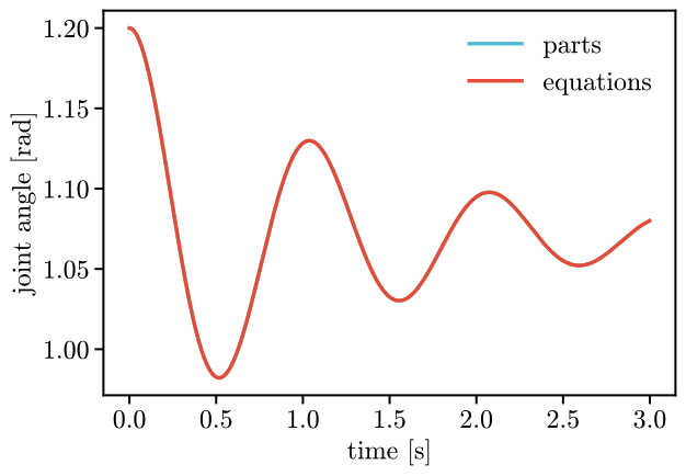
../_images/f3e3605bc743147dd9e5944a478c8dd27d4dffd05906413ac22a62a2a072d8a4.svg

The link swings 0.22 rad, and the two runs agree to better than a nanoradian. (With several joints they differ a little. The simulator’s step is linearly implicit: for the black box it linearizes the whole acceleration, for a robot of parts only the forces of its springs and dampers.) check_model takes the robot as it takes any model, and checks the mass matrix (symmetric, positive) and, when there is an energy, that a simulation never gains any:

worst = check_model(black_box())
{name: f"{error:.0e}" for name, error in worst.items()
 if name in ("mass_symmetric", "mass_positive", "energy_growth")}

{'mass_symmetric': '0e+00', 'mass_positive': '0e+00', 'energy_growth': '0e+00'}

The energy is optional. Without it the robot still simulates, plans and is controlled, but what needs the energy of the robot refuses, because the equations alone do not say what the robot dissipates: the energy of a simulation, and the passivity correction of an underactuated controller.

plant = vmc.sim.ModelPlant(black_box(energy=None), q0=[1.2])
plant.advance(0.1)  # simulating needs none
try:
    plant.energy()
except ValueError as error:
    refusal = str(error)
refusal

'the energy of a simulated robot needs the energy of the robot, and its equations of motion have none: give models.Equations an energy'

A new plant¶

A plant is anything with read, write and close. A simulated one also has a time t and advance(dt), and vmc.sim.run drives it. This wrapper applies each command one control period late, as a real loop with its communication delay does:

class Late:
    """A simulated plant that applies each command one step late."""

    def __init__(self, plant):
        self.plant, self.u = plant, np.zeros_like(plant.u)

    @property
    def t(self):
        return self.plant.t

    def read(self):
        return self.plant.read()

    def write(self, cmd):
        self.plant.write(vmc.Signals(self.t, motor_torque=self.u))
        self.u = np.array(cmd["motor_torque"], dtype=float)

    def advance(self, dt):
        self.plant.advance(dt)

    def close(self):
        self.plant.close()


arm = helyx.add_dynamics(helyx.arm("145-145-145"))
ctrl = vmc.Mechanism("ctrl")
goal = [0.1, 0.0, 0.40]  # [m]
ctrl.add("reach", vmc.LinearSpring(arm.point(s=1.0) - goal, 300.0))
ctrl.add("gravity", vmc.GravityCompensation(arm))
system = vmc.VirtualMechanismSystem(arm, ctrl)
controller = vmc.VMCController(vmc.compile(system))
late = Late(vmc.sim.ModelPlant(arm))
log = vmc.sim.run(late, controller, vmc.sim.SimClock(dt=1 / 330), T=0.5)
log.arrays()["motor_torque"].shape  # one row per step

(165, 9)

from virtualmodelcontrol import viz

viz.animate(arm, log, "extend.mp4", springs=[(1.0, goal)], trace=1.0)

The arm driven through the late plant: each torque arrives one control period late.

Tuning uses the same idea to show how the delay limits damping.

Register from another project¶

A project registers its own components, models or transmissions without changing the library, through an entry point in its pyproject.toml:

[project.entry-points."virtualmodelcontrol.plugins"]
my_project = "my_project.vmc_plugins"

Importing my_project.vmc_plugins must run its register(...) decorators. The library loads the plugins the first time a name is looked up and not found. So configuration files can use the plugins’ names (Experiments in files). Register a robot template as "robot", a simulation’s dynamics as "dynamics", an output stage as "output", a controller template as "controller" and a component as "component". Register a coordinate kind as "coordinate": a function (args, scope, path) that builds the coordinate. Register a model as "model" and a transmission as "actuation", each with to_dict and from_dict, so that vmc.models.from_dict can rebuild it from a saved description.