Hanging soft arm: identify it, reach around an obstacle¶

In this example we simulate the Helyx soft arm that hangs from its base, in two experiments. First we identify its stiffness and damping from step responses. Then its tip reaches a target around an obstacle, pulled by a force-limited spring and pushed by two repulsive fields.

The robot¶

The arm has three continuum segments, of 145, 290 and 290 mm. Three tendons run along each segment, and each tendon is wound on its own motor, so the arm has nine motors. The template describes each segment by piecewise constant curvature: its configuration is \(\Delta = (D_x, D_y, D_l)\) [m], the tendon-length differences that bend it and its elongation. The arm hangs from its base, so \(z\) points down:

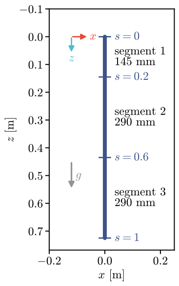
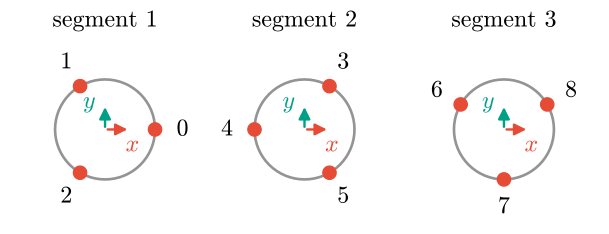
The arc parameter \(s\) runs from 0 at the base to 1 at the tip, uniformly in rest length, and arm.point(s=...) gives any point of the body. The cross-sections below, seen along each segment’s \(z\) axis, show where the tendons sit. The number beside a tendon is the index of its motor in the motor vector. A positive motor angle pulls its tendon.

Every number of the template is a Param. These are the arm’s, read from the template:

The stiffness and damping come from an identification on a real Helyx arm. Only the simulator uses them. The fit used the commanded motor torques, so the simulated arm takes each torque as the controller sends it: its efficiency is 1, the default of every template. The nine motors and their bus are in helyx.hardware("145-290-290").

Identify its stiffness and damping¶

The step experiment holds every motor at a baseline tension of 0.03 N·m, so the tendons stay taut. Each motor in turn then pulls 0.04 N·m harder for 2 s, followed by each segment’s three motors together, with 2 s back at the baseline after every pull. Three more pulls, of another size, are held out: the fit never sees them.

Steps is this experiment as a controller. It runs on any plant, here the simulated arm, and its log goes straight to identification.fit_stiffness_damping. The fit knows the arm’s masses and gravity, and fits its diagonal stiffness and damping by least squares, relative to the resting baseline. The masses are never fitted. Here the simulator plays the arm, so the result can be checked against the values it was given.

import numpy as np
import matplotlib.pyplot as plt
import virtualmodelcontrol as vmc
from virtualmodelcontrol import viz
from virtualmodelcontrol.identification import (
    Steps, fit_stiffness_damping, validate)
from virtualmodelcontrol.robots import helyx

arm = helyx.add_dynamics(helyx.arm("145-290-290"))

base = 0.03  # [N·m], on every motor
pulls = [([m], 0.04) for m in range(9)]  # [motors], [N·m] more
pulls += [([0, 1, 2], 0.04), ([3, 4, 5], 0.04), ([6, 7, 8], 0.04)]
held_out = [([0], 0.06), ([4], 0.06), ([8], 0.06)]
steps = Steps(base, pulls, held_out, hold=2.0, rest=2.0)

plant = vmc.sim.ModelPlant(arm)
clock = vmc.sim.SimClock(dt=1 / 330)
vmc.sim.run(plant, Steps(base), clock, T=3.0)  # settle under the baseline
log = vmc.sim.run(plant, steps, clock, T=steps.duration)

known = helyx.arm("145-290-290")  # masses and gravity, no stiffness
known.add("gravity", vmc.Gravity(known))
K, D = fit_stiffness_damping(known, [log], smoothing=11)

names = [rf"$D_{{{c},{i}}}$" for i in (1, 2, 3) for c in "xyl"]
x = np.arange(9)
fig, (top, bottom) = plt.subplots(2, 1, figsize=(6.4, 6.0), sharex=True)
top.bar(x - 0.2, helyx.SIM_STIFFNESS, 0.4, label="simulator")
top.bar(x + 0.2, K, 0.4, label="fitted")
top.set_ylabel("stiffness [N/m]")
top.legend(fontsize=14)
bottom.bar(x - 0.2, helyx.SIM_DAMPING, 0.4)
bottom.bar(x + 0.2, D, 0.4)
bottom.set_ylabel(r"damping [N$\cdot$s/m]")
bottom.set_xticks(x, names);

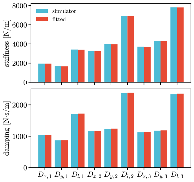
From 50 s of steps, the fit recovers every stiffness within 0.5 % and every damping within 1.0 %. On the real arm, run the same Steps through the arm’s plant (Real-time runs); the pulls must keep every tendon taut, since a slack tendon transmits nothing and the model would no longer hold.

Check it on the held-out steps¶

validate simulates the identified arm, a robot with the fitted stiffness and damping, under the torques of the held-out steps. It starts where the run is when they begin, and returns the simulated motion and its error against the logged one.

model = helyx.add_dynamics(helyx.arm("145-290-290"), stiffness=K, damping=D)
check = validate(model, log)

rows = log.arrays()  # the logged motion over the same time
inside = (rows["t"] >= check["t"][0]) & (rows["t"] <= check["t"][-1])
real = rows["q"][inside.ravel()]
t, sim = check["t"] - check["t"][0], check["q"]
moved = np.sort(np.argsort(np.ptp(real, axis=0))[-3:])  # the biggest three

fig, ax = plt.subplots(figsize=(6.4, 4.4))
for color, i in zip(viz.PALETTE, moved):
    ax.plot(t, 1e3 * (real[:, i] - real[0, i]), color=color, label=names[i])
    ax.plot(t, 1e3 * (sim[:, i] - real[0, i]), "--", color="k")
ax.set_xlabel("time [s]")
ax.set_ylabel("change of configuration [mm]")
ax.legend(fontsize=14);

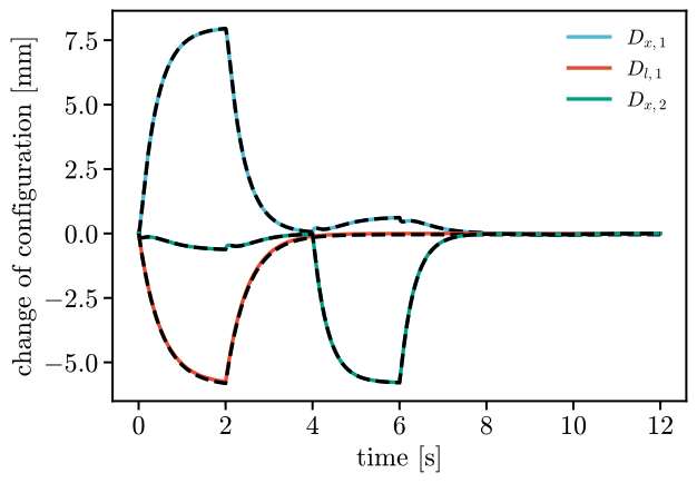
The solid lines are the logged motion of the three coordinates that move most, and the dashed lines the identified arm’s. Over the three held-out steps the arm stays within 0.05 mm (root mean square) of the logged motion on every coordinate. check["vaf"] is the share of each coordinate’s variance that the model explains; for these three, all but 0.004 % of it.

Friction¶

Static friction in the motors passes for damping. With friction=True the fit finds it too, one torque per motor that opposes its motion, and returns it after K and D:

K, D, F = fit_stiffness_damping(known, [log], smoothing=11, friction=True)

The simulated arm has no friction, and the fit finds at most 4.1e-05 N·m. A motor that stands still has no friction in the model, so a run that stops after every step shows it little. On a real arm, add a run that keeps the motors moving.

Reach around an obstacle¶

A tanh spring pulls the tip towards a target with at most 2 N, and a damper slows the tip down. An obstacle of radius 2 cm sits beside the arm’s path, and the arm must keep 2 cm clear of it. Two Gaussian fields push the arm away from the obstacle’s center. They are attached at \(s = 0.6\) and at the tip, the ends of the part that has to get past the obstacle.

target = np.array([0.20, 0.0, 0.66])  # [m]
obstacle, radius = np.array([0.155, 0.0, 0.50]), 0.02  # [m]
tip = arm.point(s=1.0)

def reach(fields):
    ctrl = vmc.Mechanism("ctrl")
    ctrl.add("reach", vmc.TanhSpring(tip - target, 60.0, 2.0))  # [N/m], [N]
    ctrl.add("damp", vmc.LinearDamper(tip, 1.0))  # [N·s/m]
    if fields:
        for i, s in enumerate((0.6, 1.0)):
            away = arm.point(s=s) - obstacle
            ctrl.add(f"avoid{i}", vmc.GaussianSpring(away, 140.0, 0.06))
    ctrl.add("gravity", vmc.GravityCompensation(arm))
    system = vmc.VirtualMechanismSystem(arm, ctrl)
    controller = vmc.VMCController(vmc.compile(system))
    clock = vmc.sim.SimClock(dt=1 / 330)
    return vmc.sim.run(vmc.sim.ModelPlant(arm), controller, clock, T=5.0)

free, avoid = reach(False), reach(True)

def draw(ax, row=None):
    disc = plt.Circle((obstacle[0], obstacle[2]), radius, color="0.4")
    ax.add_patch(disc)

viz.animate(arm, avoid, "hanging-arm-avoid.mp4",
            springs=[(1.0, target)], trace=1.0, draw=draw,
            invert=True)

fig, ax = plt.subplots(figsize=(4.6, 5.6))
kin = vmc.Kinematics(arm)
viz.draw_robot(ax, arm, np.zeros(9), color="0.85")
viz.draw_robot(ax, arm, free.arrays()["q"][-1],
               color=viz.PALETTE[5], label="reach")
viz.draw_robot(ax, arm, avoid.arrays()["q"][-1],
               label="reach and avoid")
viz.draw_goal(ax, target, label="target")
draw(ax)
ax.invert_yaxis()  # the arm hangs: z points down
viz.label_axes(ax)
ax.legend(loc="lower left", fontsize=14);

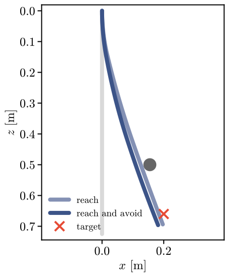
Without the fields the body passes 0.8 cm from the obstacle’s surface, closer than the 2 cm it must keep, and the tip stops 3.4 cm from the target. With them the body keeps at least 2.3 cm away, and the tip stops 4.1 cm from the target: the clearance costs a little reach. Where the fields attach and how strong they are set that trade-off.