Estimate the state of a soft arm¶

A controller needs the arm’s configuration and velocity. The encoders of the tendon motors give them through the transmission, but the tendons slacken and stretch, so the encoders drift away from the arm. In this tutorial we simulate a soft arm with three sensors, encoders, motion capture and IMUs, and fuse them with a Kalman filter that predicts with the arm’s own dynamics.

\((D_x, D_y, D_l)\) are the three coordinates of one section of the soft arm: see soft-arm kinematics.

The arm and its run¶

The arm points up. A spring pulls its tip to a goal that stays still for 0.3 s and then goes around a circle of 10 cm. We run it and keep the true \(q\) and \(v\) to compare the estimates with.

import casadi as ca
import numpy as np
import matplotlib.pyplot as plt
import virtualmodelcontrol as vmc
from virtualmodelcontrol.robots import helyx

arm = helyx.add_dynamics(helyx.arm("290-145-145"))
tip = arm.point(s=1.0)

def goal(t):  # still for 0.3 s, then a circle of 10 cm
    u = ca.fmin(ca.fmax((t - 0.3) / 1.0, 0.0), 1.0)
    r = 0.10 * (3 * u**2 - 2 * u**3)
    return ca.vertcat(r * ca.cos(4 * (t - 0.3)),
                      r * ca.sin(4 * (t - 0.3)), 0.55)

ctrl = vmc.Mechanism("ctrl")
ctrl.add("reach", vmc.LinearSpring(
    tip - vmc.Custom(goal, [vmc.Time()], dim=3), 400.0))
ctrl.add("damp", vmc.LinearDamper(tip, 5.0))
ctrl.add("gravity", vmc.GravityCompensation(arm))
system = vmc.VirtualMechanismSystem(arm, ctrl)
controller = vmc.VMCController(vmc.compile(system))

dt = 1 / helyx.CONTROL_RATE
log = vmc.sim.run(vmc.sim.ModelPlant(arm), controller,
                  vmc.sim.SimClock(dt), T=4.0)
rows = log.arrays()
t, q, v = np.ravel(rows["t"]), rows["q"], rows["v"]
u = rows["motor_torque"]  # what the motors were told at each step

What the sensors read¶

The sensors read the true motion with noise, and the library has them: Encoders, Markers, Imus and LoadCell take the true state and give a noisy reading, in the form the estimators take. The encoders read the motors, whose angles are off by a few tenths of a radian because the tendons are slack: a fraction of a millimeter of \(q\), measured below. The three markers sit at the ends of the sections, and an IMU on the base and on each section end reads its angular velocity and the direction of gravity in its own axes, with a bias on the gyros.

from virtualmodelcontrol.estimation import Encoders, Imus, Markers

n = len(t)
encoders = Encoders(arm, noise=0.01, rate_noise=0.05, slack=0.4, seed=1)
theta, theta_dot = (np.array(x) for x in
                    zip(*[encoders.read(qk, vk) for qk, vk in zip(q, v)]))

kin = vmc.Kinematics(arm)
at = [0.5, 0.75, 1.0]  # markers at the ends of the three sections
mocap = Markers(arm, at, noise=3e-4, seed=2)  # [m]
markers = np.array([mocap.read(qk) for qk in q])

sites = ["base", "seg1", "seg2", "tip"]  # an IMU on each
imus = Imus(arm, sites, bias=0.02, gyro_noise=0.005, acc_noise=0.05, seed=3)
gyro, acc = (np.array(x) for x in
             zip(*[imus.read(qk, vk) for qk, vk in zip(q, v)]))

The filter¶

KalmanFilter holds the state \((q, v)\) and its covariance. At every control step it predicts with the torques the motors were given, then updates with the measurements that came in. A Measurement(q, v, Rq, Rv, name=...) is some of the coordinates \(q\) and rates \(v\) with their covariances (variances: the square of a standard deviation), and a name. The encoders come ready: kf.encoder takes the motor angles and rates through the transmission. The markers go through Inversion, which finds the \(q\) that puts the arm’s points on them, and the markers’ \(v\) comes from VelocityFilter, a low-passed difference of consecutive \(q\). The IMUs’ \((D_x, D_y)\) and their rates come from ImuFilter, which is observed on those coordinates only. The markers and the IMUs run at a third of the control rate, as real ones do. In kf.encoder(theta, theta_dot, 1.5e-3**2, 1e-2**2) the last two numbers are the variances of the \(q\) and the \(v\) that the readings give: 1.5 mm and 1 cm/s. kf.reset(q0) starts the filter at rest at the configuration q0, here the one that the first encoder reading gives (the y of that measurement is its values). A sensor that sees combinations of the coordinates, such as tendon lengths or the motors of a robot with fewer motors than joints, gives its matrix (\(m \times n\)) instead: it reads matrix @ q and matrix @ v, and kf.encoder does this by itself for such a robot (see Robots with fewer motors than joints).

from virtualmodelcontrol.estimation import (
    ImuFilter, Inversion, KalmanFilter, Measurement, VelocityFilter)

Q = np.diag([1e-12] * 9 + [1e-5] * 9)  # the model's error, on q then v
every = 3  # steps between two frames of the markers, or of the IMUs

def estimate(sensors, markers=markers, gate=40.0, lost=()):
    """Run the filter over the recorded readings; the frames in ``lost``
    never arrive. ``gate`` is explained in "Outliers and dropouts"."""
    kf = KalmanFilter(system, dt, Q=Q, P0=1e-4, gate=gate)
    inversion = Inversion(arm, at)
    velocity = VelocityFilter(every * dt)
    imu = ImuFilter(arm)
    imu.calibrate(gyro[:90], acc[:90])  # the arm is still at first
    kf.reset(kf.encoder(theta[0], None, 1.5e-3**2).y)  # encoders start
    out, missing = [np.concatenate([kf.q, kf.v])], 0
    for k in range(1, n):
        kf.predict(u[k - 1])
        seen = [kf.encoder(theta[k], theta_dot[k], 1.5e-3**2, 1e-2**2)]
        asked = ["encoder"]
        if "mocap" in sensors and k % every == 0:
            asked.append("mocap")
            if k not in lost:
                qm = inversion(markers[k])
                seen.append(Measurement(qm, velocity.update(qm), 0.5e-3**2,
                                        5e-2**2, name="mocap"))
        if "imu" in sensors and k % every == 1:
            asked.append("imu")
            qi, vi = imu.update(gyro[k], acc[k], every * dt)
            seen.append(Measurement(qi, vi, 2e-3**2, 5e-2**2,
                                    observed=imu.observed, name="imu"))
        kf.update(seen, expected=asked)
        missing += len(kf.missing)
        if "mocap" in kf.rejected or "mocap" in kf.missing:
            velocity.reset()  # the next frame has nothing to differ from
            inversion.reset(kf.q)  # and its fit starts from the estimate
        out.append(np.concatenate([kf.q, kf.v]))
    return np.array(out), kf.rejected_total, missing

The filter’s model is the simulated arm itself, so Q can be small. On a real arm, Q is where the model’s errors go. P0 is the covariance of the starting state. The covariances of the measurements are the noise we gave the sensors, with the slack counted in for the encoders: 1.5 mm.

predict linearizes the arm’s dynamics at the estimate. That is exact for a linear robot and close for an arm whose state is known to a few millimeters. For a state that is much less certain, build the filter with KalmanFilter(system, dt, unscented=True). Its predict sends sigma points of the estimate, \(\sqrt 3\) (about 1.7) standard deviations out, through substeps steps of the arm’s own integrator, and takes the mean and the covariance of where they land, so both follow the arm’s nonlinearity. It sends \(4n + 1\) points for \(n\) coordinates, and a step took 136 times as long as the linearized one here. The sensors are fused as before, since they are linear in \(q\) and \(v\).

One estimate, three sensors¶

We run the filter with each combination of sensors and compare with the true state, after the first second.

truth = np.hstack([q, v])
combos = {"encoders": ("encoder",),
          "encoders + IMUs": ("encoder", "imu"),
          "encoders + markers": ("encoder", "mocap"),
          "all three": ("encoder", "mocap", "imu")}
runs = {name: estimate(sensors) for name, sensors in combos.items()}

def rms(error):  # [mm] and [mm/s]
    return 1e3 * np.sqrt(np.mean(error[t > 1.0] ** 2))

print(f"{'sensors':20s}{'q [mm]':>10s}{'v [mm/s]':>10s}")
for name, (est, _, _) in runs.items():
    e = est - truth
    print(f"{name:20s}{rms(e[:, :9]):10.2f}{rms(e[:, 9:]):10.2f}")

sensors                 q [mm]  v [mm/s]
encoders                  0.33      0.32
encoders + IMUs           0.28      0.28
encoders + markers        0.09      0.12
all three                 0.09      0.11

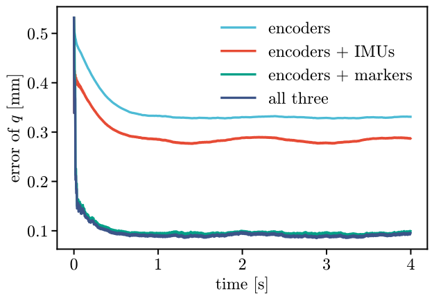
The encoders alone are off by 0.33 mm: they read the slack. The markers anchor the estimate to the arm: with them the error is 0.09 mm, 3.5 times smaller, and the velocity improves too, 2.8 times. The IMUs help less. They see how the sections bend and not how long they are, and the markers see all of it. On an arm with no markers they still cut the error of the encoders.

Outliers and dropouts¶

Markers jump when a camera swaps two of them, and frames get lost when one is hidden. The filter takes both. Each measurement has to pass the gate before it is used: its innovation, how far it is from what the filter expected, measured in the measurement’s own standard deviations, must stay below a limit. The default limit is \(d^2 = 40\), about the 99.8 % bound of a chi-squared distribution with the 18 values of a reading of \(q\) and \(v\), so at most about two good readings in a thousand are turned away. In this run, with nothing wrong, the gate turned away 0 of the 2198 readings. A real outlier is far outside the limit. We move all three markers by 10 cm along each axis for two frames, and run the filter with the gate and without it:

bad = markers.copy()
bad[700:706] += 0.1  # [m], two frames of the markers
both = ("encoder", "mocap")
gated = estimate(both, markers=bad)
ungated = estimate(both, markers=bad, gate=None)
window = (t > 2.1) & (t < 2.7)
fits = {"gate": gated, "no gate": ungated}
worst = {name: round(float(1e3 * abs((est - truth)[window, :9]).max()), 2)
         for name, (est, _, _) in fits.items()}
worst, gated[1], ungated[1]  # the worst error [mm], and the frames rejected

({'gate': 0.32, 'no gate': 1.1}, 2, 0)

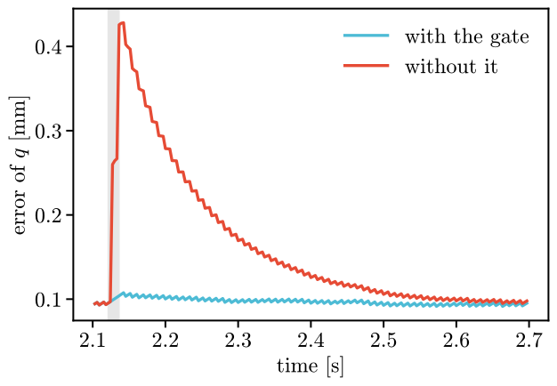
With the gate the worst error is 0.32 mm, without it 1.10 mm. The gate turned 2 frames away: the two that were wrong, and 0 good ones, as in the run without the outlier. After a rejected or missing frame, estimate resets the velocity filter, which has no previous frame to differ from, and the inversion, which starts from the estimate: neither keeps the jump.

A lost frame is not a rejected one. update(..., expected=[...]) names the sensors that should have come: those that did not are in kf.missing, and those the gate turned away are in kf.rejected. With no frame of the markers for a third of a second the filter keeps going on the encoders and the model:

dropout = estimate(both, lost=set(range(600, 700)))
shown = (t > 1.0)
dropped = 1e3 * np.sqrt(np.mean((dropout[0] - truth)[shown, :9] ** 2))
print(f"{dropout[2]} frames missing, error {dropped:.2f} mm")

34 frames missing, error 0.11 mm

The error with the frames lost is 0.11 mm. With every frame it was 0.09 mm, and with the encoders alone 0.33 mm: the encoders and the model carry the filter through the gap, and it takes the markers up again when they come back.

A window of readings¶

The filter keeps one state and its covariance and forgets the readings once it has used them. MovingHorizon keeps the last few steps instead. At every step it finds the states of the window that agree best with all the readings in it, with the arm’s own dynamics (up to the process noise Q) and with the estimate the window started from, each weighted by its covariance. When the window slides on, the state before it goes one step of an extended Kalman filter, so that what the window forgets is not lost. It takes the same Measurements as the filter, and encoder the same way:

from virtualmodelcontrol.optimization import MovingHorizon

first = 330  # the first second only: the window costs more than a filter
mhe = MovingHorizon(system, dt, window=3, Q=Q, P=1e-4)
inversion = Inversion(arm, at)
mhe.reset(mhe.encoder(theta[0], None, 1.5e-3**2).y)
states = []
for k in range(1, first):
    seen = [mhe.encoder(theta[k], theta_dot[k], 1.5e-3**2, 1e-2**2)]
    if k % every == 0:
        qm = inversion(markers[k])
        seen.append(Measurement(qm, None, 0.5e-3**2, name="mocap"))
    states.append(mhe.step(u[k - 1], seen))
states = np.array(states)

With the encoders and the markers, from half a second to one second, the window’s error in \(q\) is 0.09 mm and the filter’s 0.10 mm. They are close, as they must be: this arm stays near one pose, and for a linear robot the window is the filter. The window pays off where the arm is not near a pose, or the readings are not Gaussian, and a longer window follows them better. It costs more, since each step solves a least squares of every state in the window, and that grows with the window. It is for offline fits, for slow robots and for checking a filter. iterations bounds the solver, and cost and P tell how well the last window fits and how sure the estimate is.

On a real arm¶

The numbers here come from sensors we simulated. For a real arm, take the noise of each sensor from a recording of the arm held still, set Q by trying values until the estimate is smooth and still follows a quick move, and look at kf.rejected_total: a gate that turns away many frames means the covariances are too small, or a sensor is wrong.

The markers’ positions must be in the arm’s base frame: Inversion takes positions as rows of \((x, y, z)\) in that frame, so a motion-capture system that reports them in the room needs one change of frame first, \(R^\top (p - b)\) with the base’s rotation \(R\) and position \(b\). From the neutral configuration Inversion finds the soft arm up to 0.6 rad of bend in each section, and it keeps its last result as the start of the next fit; after a long gap, give it q0.

Take it to the robot¶

On the robot the filter sits in the loop that reads the sensors, with nothing from vmc.sim. At each control period it predicts with the torques last sent, then fuses what came in, and the controller reads \(q\) and \(v\) from it. Here is that period for the encoders alone, with the readings of the recorded run standing in for the robot’s:

kf = KalmanFilter(system, dt, Q=Q, P0=1e-4)
kf.reset(kf.encoder(theta[0], None, 1.5e-3**2).y)

def estimate_step(command, theta, theta_dot):
    """The torques last sent and the encoders' reading, in; q and v, out."""
    kf.predict(command)
    kf.update([kf.encoder(theta, theta_dot, 1.5e-3**2, 1e-2**2)])
    return kf.q, kf.v

q_hat, v_hat = estimate_step(u[0], theta[1], theta_dot[1])