Plan around an obstacle¶

In this tutorial the optimizer plans the soft arm’s swap around a sphere: it chooses the strength of a repulsive field with the spring’s stiffness, then which of five fields to keep.

The arm and the controller in place¶

They are those of Optimizing a virtual mechanism: the hanging soft arm, held by a soft spring, which we let settle first, and the same horizon, swap time and number of nodes:

import numpy as np
import matplotlib.pyplot as plt
import virtualmodelcontrol as vmc
from virtualmodelcontrol import optimization as opt
from virtualmodelcontrol.robots import helyx

arm = helyx.add_dynamics(helyx.arm("145-290-290"))  # hangs from its base
tip = arm.point(s=1.0)
kin = vmc.Kinematics(arm)

hold = vmc.Mechanism("hold")  # the controller in place
hold.add("drag", vmc.LinearSpring(tip - [0.01, 0.0, 0.70], 10.0))
hold.add("damp", vmc.LinearDamper(tip, 2.0))
hold.add("gravity", vmc.GravityCompensation(arm))
held = vmc.VirtualMechanismSystem(arm, hold)

plant = vmc.sim.ModelPlant(arm)
settle = vmc.VMCController(vmc.compile(held))
vmc.sim.run(plant, settle, vmc.sim.SimClock(1 / 330), T=12.0)
q0 = plant.q.copy()  # the arm at rest under the spring in place
HORIZON, SWAP, NODES = 5.0, 2.0, 21  # [s], [s]

Around an obstacle¶

A sphere of radius 2 cm stands by the arm’s path to a farther target. We add a repulsive Gaussian field on the arm, at \(s = 0.6\), that pushes that point away from the sphere’s center. The optimizer chooses its strength together with the spring’s stiffness. SphereDistance is the signed distance from a point to the sphere’s surface, and a Bound keeps it above 2 cm at every node, for 41 points along the arm:

goal = [0.20, 0.0, 0.66]  # [m]
ball, R = [0.15, 0.0, 0.50], 0.02  # the sphere's center and radius [m]

k = vmc.Param("k", 20.0, bounds=(1.0, 300.0), scope="stage")  # [N/m]
A = vmc.Param("A", 50.0, bounds=(0.0, 500.0), scope="stage")  # [N/m]
around = vmc.Mechanism("around")
around.add("pull", vmc.TanhSpring(tip - goal, k, 2.0))
around.add("push", vmc.GaussianSpring(arm.point(s=0.6) - ball, A,
                                      0.06))  # strength A, width 0.06 m
around.add("damp", vmc.LinearDamper(tip, 2.0))
around.add("gravity", vmc.GravityCompensation(arm))
detour = vmc.VirtualMechanismSystem(arm, around)

body = [arm.point(s=s) for s in np.linspace(0.0, 1.0, 41)]
clear = vmc.Stack(*[vmc.SphereDistance(p, ball, R) for p in body])


def plan_for(terms=(), scales=(1, 1, 1)):
    problem = opt.Problem(detour)
    problem.add(opt.Collocation(q0, HORIZON, NODES, initial=held,
                                transition=SWAP, scales=scales))
    problem.free("around.pull.stiffness", "around.push.strength")
    problem.add(opt.Effort(0.2))
    problem.add(opt.Cost(tip - goal, t_from=SWAP, name="reach"))
    for term in terms:
        problem.add(term)
    return problem.solve()


straight = plan_for()  # the sphere is not in the problem
safe = plan_for([opt.Bound(clear, lower=0.02, name="clear")])

The optimizer finds the Params by their place in the system, whatever the Python variables are called: around.pull.stiffness is the stiffness of the element pull of the mechanism around. Without the bound the optimizer has no reason to push: it keeps the field off and takes the cheapest spring. With the bound, it switches the field on. We run both plans on the simulated arm, as before, and follow the arm’s closest distance to the sphere’s surface:

def swap_to(plan):
    controller = vmc.VMCController(vmc.compile(detour))
    plan.apply(controller)
    swap = vmc.control.SwapController(vmc.VMCController(vmc.compile(held)))
    swap.swap(controller, SWAP)
    sim = vmc.sim.ModelPlant(arm, q0=q0)
    return vmc.sim.run(sim, swap, vmc.sim.SimClock(1 / 330), T=HORIZON)


def gap(q):  # [cm] from the arm to the sphere's surface, at its closest
    points = [kin.position(q, s) for s in np.linspace(0.0, 1.0, 101)]
    return 100 * (min(np.linalg.norm(p - ball) for p in points) - R)


runs = {"without the bound": swap_to(straight).arrays(),
        "with the bound": swap_to(safe).arrays()}

fig, ax = plt.subplots()
for name, rows in runs.items():
    ax.plot(rows["t"][::5], [gap(q) for q in rows["q"][::5]], label=name)
ax.plot(safe.t, [gap(q) for q in safe.q], "o", label="plan")
ax.axhline(2.0, color="gray", linestyle=":")
ax.set_xlabel("time [s]")
ax.set_ylabel("distance to the sphere [cm]")
ax.legend(loc="upper right", fontsize=18);

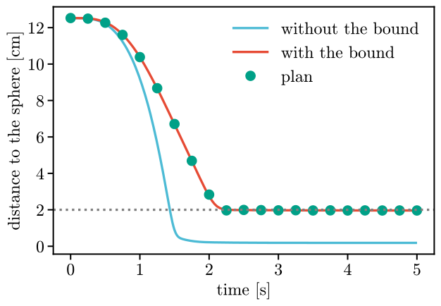
../_images/69373e3ac0aea2782a975ad1aa8414b0c9e7b29314cbf299be94609da1882a3c.svg

Without the bound the arm passes 0.2 cm from the sphere. With it, the optimizer chose a stiffness of 126 N/m and a field of 230 N/m (it was 0 before), and the simulated arm keeps 1.96 cm: the bound holds at the nodes and at 41 points of the arm, and between them the arm can come a little closer. The dotted line marks 2 cm.

Do the scales matter?¶

Not on this problem. With other scales, (0.05, 0.3, 20), the solver finds the same plan (the scales are the typical sizes of q, v and a):

other = plan_for([opt.Bound(clear, lower=0.02, name="clear")],
                 scales=(0.05, 0.3, 20.0))
for result in (safe, other):
    print(result.iterations, {n: round(v.item(), 1)
                              for n, v in result.params.items()})

22 {'around.pull.stiffness': 125.6, 'around.push.strength': 230.0}
29 {'around.pull.stiffness': 125.6, 'around.push.strength': 230.0}

Both reach the same stiffness and strength, in 22 and 29 iterations. This is a property of the problem. The scales change the solver’s path, and a problem with several local optima can end in another one with another scaling, so when you plan a new task, try two scalings and compare.

Which fields to keep¶

We put the field at \(s = 0.6\) ourselves. Let the optimizer choose among five places instead. Gated multiplies an element’s force by a gate between 0 and 1, a live Param like the others, and Sparsity adds the sum of the gates to the cost: an element that does not pay for itself closes. We free the gates and the spring’s stiffness:

places = [0.3, 0.45, 0.6, 0.75, 0.9]  # candidate fields, along the arm [s]

fields = vmc.Mechanism("fields")
fields.add("pull", vmc.TanhSpring(tip - goal, k, 2.0))
fields.add("damp", vmc.LinearDamper(tip, 2.0))
for i, s in enumerate(places):
    push = vmc.GaussianSpring(arm.point(s=s) - ball, 200.0, 0.06)
    fields.add(f"push{i}", vmc.Gated(push, 0.5))  # open halfway
fields.add("gravity", vmc.GravityCompensation(arm))
choice = vmc.VirtualMechanismSystem(arm, fields)


def choose(weight):
    problem = opt.Problem(choice)
    problem.add(opt.Collocation(q0, HORIZON, NODES, initial=held,
                                transition=SWAP))
    problem.free("fields.pull.stiffness", "fields.push*.gate")
    problem.add(opt.Effort(0.2))
    problem.add(opt.Cost(tip - goal, t_from=SWAP, name="reach"))
    problem.add(opt.Bound(clear, lower=0.02, name="clear"))
    if weight:
        problem.add(opt.Sparsity(weight, "fields.push*.gate"))
    return problem.solve()


many, few = choose(0.0), choose(3e-3)
gates = {name: [plan.params[f"fields.push{i}.gate"].item()
                for i in range(5)]
         for name, plan in (("no sparsity", many), ("sparsity", few))}

fig, ax = plt.subplots()
x = np.arange(5)
for dx, (name, values) in zip((-0.2, 0.2), gates.items()):
    ax.bar(x + dx, values, 0.4, label=name)
ax.set_xticks(x, [f"{s:g}" for s in places])
ax.set_xlabel("place of the field along the arm [s]")
ax.set_ylabel("gate")
ax.legend(fontsize=18);

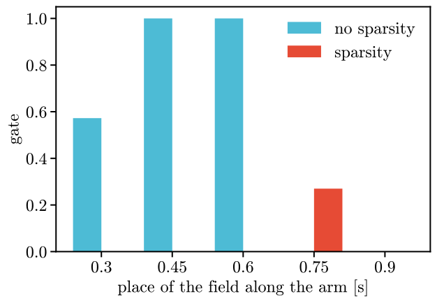
../_images/36a976b9ad55896469db457a62a08e217f7bea065b4b0288c3e9d8e288a7de53.svg

Without the term, 3 fields are open. With it, one is: the field at s = 0.75, with a gate of 0.27 and a spring of 69 N/m. A gate is a number, not a switch: a gate of 0.3 is a weaker field. The weight decides how much a field must earn to stay. Structure problems are rough, since elements switch on and off, and another weight, another start or other scales can end in another structure, so solve a few and compare.

To plan again at every step from the measured state, see Model predictive control, and for motions that repeat, Plan periodic motions and virtual states.