Components¶

In this tutorial we list the components of the library, try a damper that works one way, and compare how the springs push. A component acts on a coordinate.

The list¶

A component acts on one coordinate \(y\), and it is one of four kinds:

• storage: an energy \(V(y)\) and the force \(f = -\partial V / \partial y\) (springs; gravity on the robot);

• dissipation: a force with \(f \cdot \dot y \le 0\) (dampers);

• inertance: a mass or inertia \(M\), with kinetic energy \(\tfrac12 \dot y^\top M \dot y\);

• source: a force whose power \(f \cdot \dot y\) is counted apart in the energy balance (force sources, gravity compensation; see Energy and passivity).

Each force reaches the robot through its coordinate’s Jacobian: \(\dot y = J v\) and \(\tau = J^\top f\). The motors then receive the torques \(u\) with \(B(q)\,u = \tau\), where \(B\) comes from the robot’s transmission. The conventions give the signs. These are the components of the library:

The arguments are listed in the order the constructors take them, with the symbols of the formulas; the keyword names (stiffness, damping, max_force, …) are in the API reference.

An Inertance on a difference of two coordinates is an inerter: a mass between them, with a force \(M\,(\ddot y_1 - \ddot y_2)\) that opposes their relative acceleration. A LimitSpring on a slice of the joints, with a lower and an upper bound per joint, gives all of them soft limits.

For the sigmoid and polynomial springs, \(d\) is the size of each axis of \(y\), or its norm with element_wise=False. A new component only needs its energy or its force (Extend the library).

A damper that works one way¶

A DiodeDamper(y, D, sign) damps one direction of motion: the positive rates for sign=1, the negative ones for sign=-1, and never adds energy. A mass of 1 kg on a spring of 100 N/m, let go at 0.1 m, swings back and forth. Damped both ways it loses its swing at the same rate on each side (with 2 N·s/m). Damped on the way up only, with twice that, because it works on half of each swing, it still swings down almost as far as it started:

import numpy as np
import matplotlib.pyplot as plt
import virtualmodelcontrol as vmc

def swing(damper):
    """The height of a mass on a spring, let go at 0.1 m."""
    mass = vmc.Mechanism("mass", model=vmc.models.JointSpace(1, unit="m"))
    y = mass.joint(0)
    mass.add("inertia", vmc.Inertance(y, 1.0))
    mass.add("spring", vmc.LinearSpring(y, 100.0))
    mass.add("damper", damper(y))
    plant = vmc.sim.ModelPlant(mass, q0=[0.1], max_step=1e-4)
    out = []
    for _ in range(300):
        plant.advance(0.01)
        out.append(plant.q[0])
    return np.array(out)

swings = {"both ways": swing(lambda y: vmc.LinearDamper(y, 2.0)),
          "upwards only": swing(lambda y: vmc.DiodeDamper(y, 4.0))}

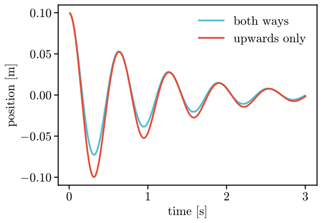
Its first swing down reaches -0.100 m.

The springs side by side¶

We put six springs on six independent coordinates of a test mechanism, compile them, and read their forces over a range of deflections.

Show code cell source

Hide code cell source

bar = vmc.Mechanism("bar", model=vmc.models.JointSpace(6, unit="m"))
y = [bar.joint(i) for i in range(6)]  # six deflections [m]
springs = {
    "LinearSpring": vmc.LinearSpring(y[0], 10.0),
    "TanhSpring": vmc.TanhSpring(y[1], 10.0, 0.6),
    "GaussianSpring": vmc.GaussianSpring(y[2], 40.0, 0.05),
    "SigmoidSpring": vmc.SigmoidSpring(y[3], 2.0, 20.0, 0.1, 60.0),
    "PolynomialSpring": vmc.PolynomialSpring(y[4], 10.0, 2, 0.1),
    "LimitSpring": vmc.LimitSpring(y[5], 10.0, -0.1, 0.1),
}
probe = vmc.Mechanism("springs")
for name, spring in springs.items():
    probe.add(name, spring)
law = vmc.compile(vmc.VirtualMechanismSystem(bar, probe))

d = np.linspace(-0.3, 0.3, 241)  # [m]
q, v, z = np.tile(d, (6, 1)), np.zeros((6, 1)), np.zeros((0, 1))
# law.tau(q, v, z, p, t) is the torque; map evaluates it at every column
forces = law.tau.map(d.size)(q, v, z, law.live_values(), 0.0).full()

fig, axes = plt.subplots(3, 2, figsize=(6.4, 7.6), sharex=True)
for ax, name, f in zip(axes.flat, springs, forces):
    ax.axhline(0.0, color="0.85", lw=1)
    ax.axvline(0.0, color="0.85", lw=1)
    ax.plot(d, f)
    ax.set_title(name)
for ax in axes[-1]:
    ax.set_xlabel("$y$ [m]")
for ax in axes[:, 0]:
    ax.set_ylabel("$f$ [N]")

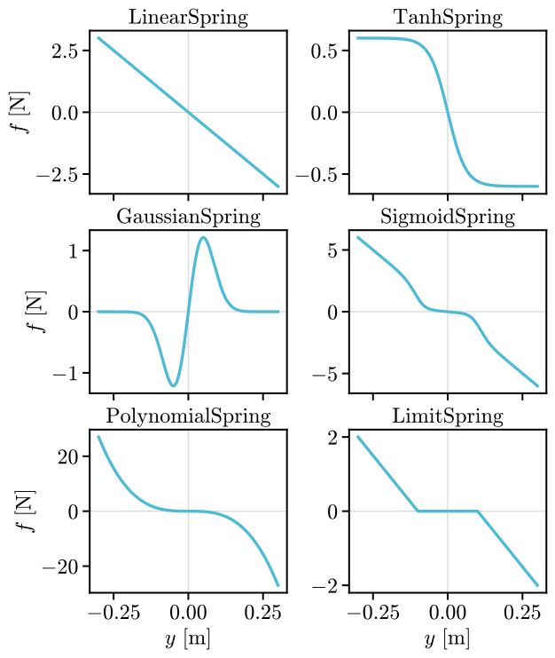
The tanh spring saturates at its maximum force. The Gaussian spring pushes away only near \(y = 0\), around an obstacle. The sigmoid and polynomial springs stiffen with distance. The limit spring stays at zero inside its range. On a 3D coordinate the tanh spring saturates each axis on its own. To bound the force along one direction, put it on a Projection.