
Kinematics and tool springs on the UR5
In this tutorial we compute the position and rotation of the UR5’s tool, and its Jacobians and Hessian, which we check against finite differences. Then we compute the joint stiffness that a spring at the tool produces, and put a spring on the tool’s orientation and one along the tool’s own axes.
The arm
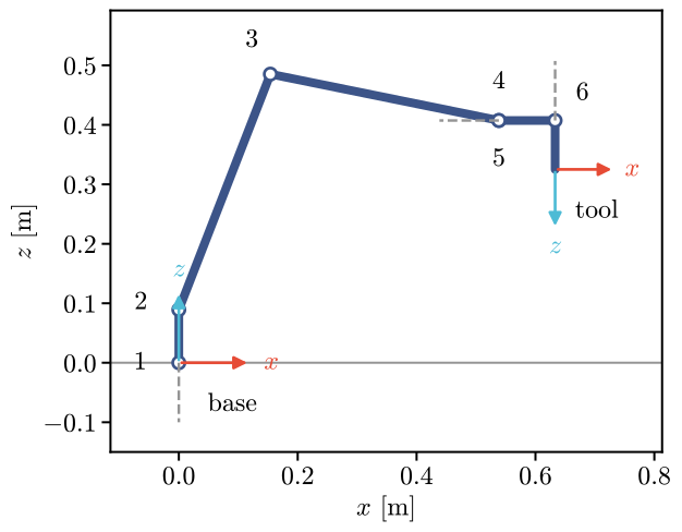
The UR5 template is built from the arm’s Denavit-Hartenberg table, with the flange as the site
tool. Its six joints are position-controlled on the real arm, so here we use its kinematics
only.
Joint |
Name |
d [m] |
a [m] |
α [rad] |
|---|---|---|---|---|
1 |
|
0.089159 |
0 |
π/2 |
2 |
|
0 |
-0.425 |
0 |
3 |
|
0 |
-0.39225 |
0 |
4 |
|
0.10915 |
0 |
π/2 |
5 |
|
0.09465 |
0 |
−π/2 |
6 |
|
0.0823 |
0 |
0 |
Positions and rotations
vmc.Kinematics evaluates any site of a robot at a configuration: its position [m], its
rotation, its Jacobians and its Hessian, all exact, by automatic differentiation.
import numpy as np
import matplotlib.pyplot as plt
import virtualmodelcontrol as vmc
from virtualmodelcontrol import viz
from virtualmodelcontrol.robots import ur5

arm = ur5.arm()
kin = vmc.Kinematics(arm)
q = np.array([0.3, -1.1, 1.4, -1.6, -1.4, 0.2])  # [rad]
kin.position(q, "tool"), kin.rotation(q, "tool").round(3)
(array([-0.57217386, -0.30588932,  0.24853857]),
 array([[-0.06 ,  0.951,  0.302],
        [ 0.992,  0.089, -0.084],
        [-0.107,  0.295, -0.95 ]]))
Jacobians
The Jacobian \(J\) maps joint velocities to the tool’s velocity, \(\dot p = J \dot q\), and the angular Jacobian \(J_\omega\) to its angular velocity, \(\omega = J_\omega \dot q\), in the base frame. Central finite differences of the position and the rotation agree with both:
h, eye = 1e-6, np.eye(6)
J, Jw = kin.jacobian(q, "tool"), kin.angular_jacobian(q, "tool")
R = kin.rotation(q, "tool")
J_fd, Jw_fd = np.zeros((3, 6)), np.zeros((3, 6))
for i in range(6):
    up, down = q + h * eye[i], q - h * eye[i]
    dp = kin.position(up, "tool") - kin.position(down, "tool")
    J_fd[:, i] = dp / (2 * h)
    dR = (kin.rotation(up, "tool") - kin.rotation(down, "tool")) / (2 * h)
    W = dR @ R.T  # the skew matrix of the angular velocity
    Jw_fd[:, i] = [W[2, 1], W[0, 2], W[1, 0]]
print("J error:", np.abs(J - J_fd).max())
print("Jw error:", np.abs(Jw - Jw_fd).max())
J error: 1.2666956372697769e-10
Jw error: 1.5608370151909412e-10
Hessians
The Hessian \(H_k = \partial^2 p_k / \partial q^2\) is the second derivative of each coordinate of the position. It tells how the Jacobian changes, and gives a second-order prediction of the position:
H = kin.hessian(q, "tool")  # (3, 6, 6)
direction = np.ones(6) / np.sqrt(6)
steps = np.logspace(-4, -1, 13)  # [rad]
first, second = [], []
for s in steps:
    dq = s * direction
    exact = kin.position(q + dq, "tool")
    linear = kin.position(q, "tool") + J @ dq
    first.append(np.linalg.norm(exact - linear))
    second.append(np.linalg.norm(exact - linear - 0.5 * H @ dq @ dq))

fig, ax = plt.subplots()
ax.loglog(steps, first, "o-", label=r"$p + J\,\delta q$")
label = r"$+ \frac{1}{2}\,\delta q^\top H\,\delta q$"
ax.loglog(steps, second, "s-", label=label)
ax.set_xlabel(r"step $\|\delta q\|$ [rad]")
ax.set_ylabel("prediction error [m]")
ax.legend();
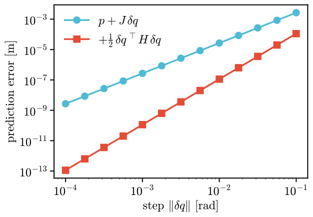
The first-order error falls with the square of the step and the second-order one with its cube, as they should: the slopes of the lines are 2.0 and 3.0.
The stiffness a tool spring gives the joints
A spring of stiffness \(K\) between the tool and a goal pushes with \(f = -K (p - g)\), which the joints feel as \(\tau = J^\top f\). Its joint stiffness, \(-\partial\tau/\partial q\), has two parts: \(J^\top K J\), and a term from the Hessian that appears as soon as the spring is stretched, \(-\sum_k f_k H_k\). A finite difference of \(\tau\) confirms the sum:
K = 500.0 * np.eye(3)  # [N/m]
goal = kin.position(q, "tool") + [0.05, 0.0, -0.03]  # [m]

def tool_torque(q):
    f = -K @ (kin.position(q, "tool") - goal)
    return kin.jacobian(q, "tool").T @ f

f = -K @ (kin.position(q, "tool") - goal)
geometric = J.T @ K @ J
stretched = -np.einsum("k,kij->ij", f, H)
fd = -np.column_stack(
    [(tool_torque(q + h * e) - tool_torque(q - h * e)) / (2 * h)
     for e in eye])
print("error with both terms:", np.abs(geometric + stretched - fd).max())
print("error without the Hessian term:", np.abs(geometric - fd).max())
error with both terms: 3.58112117737619e-08
error without the Hessian term: 17.60478653212016
A spring on the tool’s orientation
The tool’s orientation is a coordinate too. OrientationError is the rotation vector \(\phi\)
that takes a goal orientation to the tool’s, in the goal’s axes, and a spring on it is a
rotational spring of stiffness \(K_r\) [N·m/rad], with energy \(\tfrac12 \phi^\top K_r \phi\). The
joints feel the torque \(-(\partial\phi/\partial q)^\top K_r \phi\). The derivative of \(\phi\) is
not the angular Jacobian \(J_\omega\): the two agree near the goal only. The library differentiates
the error exactly, so the torque is the gradient of the energy at any error. A compiled law holds
CasADi functions of (q, v, z, p, t): the configuration, the velocity, the controller’s virtual
state (none here, it has none), its live values and the time. law.tau gives the torque on
each joint and law.energy the stored and the kinetic energy. Here the goal is 0.8 rad from the
tool (vmc.math.exp_so3 turns a rotation vector into a rotation matrix, and log_so3 turns it
back):
Kr = np.diag([30.0, 20.0, 10.0])  # [N·m/rad], in the goal's axes
axis = np.array([0.3, -0.5, 0.8]) / np.linalg.norm([0.3, -0.5, 0.8])
none = np.zeros(0)

def spring(angle):
    """The compiled spring, and the goal orientation ``angle`` away."""
    R_goal = R @ vmc.math.exp_so3(angle * axis).T
    error = vmc.OrientationError(arm.model, "tool",
                                 goal=vmc.math.log_so3(R_goal))
    ctrl = vmc.Mechanism("ctrl")
    ctrl.add("turn", vmc.LinearSpring(error, Kr))
    return vmc.compile(vmc.VirtualMechanismSystem(arm, ctrl)), R_goal

def torque(law, q):
    return np.array(law.tau(q, 0 * q, none, law.live_values(), 0.0)).ravel()

def energy(law, q):
    return float(law.energy(q, 0 * q, none, law.live_values(), 0.0)[0])

law, R_goal = spring(0.8)
rise = [energy(law, q + h * e) - energy(law, q - h * e) for e in eye]
gradient = np.array(rise) / (2 * h)
print("torque + gradient of the energy:",
      np.abs(torque(law, q) + gradient).max())
torque + gradient of the energy: 1.2768044399535938e-09
The torque from \(J_\omega\) instead, \(-(R_\text{goal}^\top J_\omega)^\top K_r \phi\), is the right one only near the goal. We compare the two as the goal moves away:
angles = np.linspace(0.05, 2.2, 12)  # [rad]
share = []
for angle in angles:
    law, R_goal = spring(angle)
    phi = vmc.math.log_so3(R_goal.T @ R)
    naive = -(R_goal.T @ Jw).T @ Kr @ phi
    exact = torque(law, q)
    share.append(np.abs(naive - exact).max() / np.abs(exact).max())

fig, ax = plt.subplots()
ax.plot(angles, 100 * np.array(share), "o-")
ax.set_xlabel("angle from the goal [rad]")
ax.set_ylabel(r"error of the $J_\omega$ torque [%]");
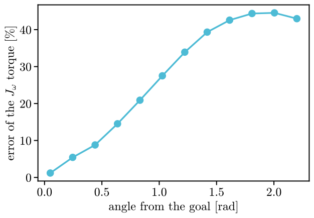
At 1.4 rad the torque from \(J_\omega\) is off by 39 %. A damper on the same coordinate acts on the rate of the error, which near the goal is the tool’s angular velocity relative to the goal.
A spring along the tool’s axes
A stiffness is often wanted along the tool’s own axes: stiff across a tool, soft along it.
vmc.InFrame(c, model, site) is a vector coordinate \(c\) taken along the axes of a frame,
\(R^\top c\), and vmc.FromFrame does the opposite. A spring \(K\) on InFrame(tool - goal, ...)
has the stiffness \(R K R^\top\) in the base frame, which turns with the tool. At the goal it gives
the joints \(J^\top R K R^\top J\), as a finite difference of the torque confirms:
Kt = np.diag([400.0, 40.0, 400.0])  # [N/m] along the tool's x, y and z
goal = kin.position(q, "tool")  # the tool is on its goal
ctrl = vmc.Mechanism("ctrl")
along = vmc.InFrame(arm.point("tool") - goal, arm.model, "tool")
ctrl.add("hold", vmc.LinearSpring(along, Kt))
law = vmc.compile(vmc.VirtualMechanismSystem(arm, ctrl))
pushes = [torque(law, q + h * e) - torque(law, q - h * e) for e in eye]
fd = -np.column_stack(pushes) / (2 * h)
print("error:", np.abs(J.T @ R @ Kt @ R.T @ J - fd).max())
error: 2.9995277373018325e-08
Moving the joints
A log needs only the time and the configurations, so viz.animate can replay any motion, even
one that is not simulated. Here is a smooth sweep of three joints:
t = np.linspace(0.0, 4.0, 401)  # [s]
sweep = np.outer(np.sin(np.pi * t / 2), [0.5, 0.4, -0.5, 0.0, 0.0, 0.0])
log = {"t": t[:, None], "q": q + sweep}
viz.animate(arm, log, "kinematics.mp4", plane="xz", trace="tool")