Model predictive control¶

In this tutorial a controller looks ahead. At every step it plans the stiffness and the reference of a virtual spring over the next second, applies the first part of the plan, and plans again from where the robot is. We regulate a mass to a goal with a spring that cannot pull harder than 5 N, then let a Tank pay for the changes.

The mass and its spring¶

A mass of 1 kg with some friction, under a spring-damper controller. The spring saturates at 5 N, which is the cap on the effort. Its stiffness and its reference are Params with bounds, and scope="stage" makes them live, so that a running controller can change them:

import numpy as np
import matplotlib.pyplot as plt
import virtualmodelcontrol as vmc
from virtualmodelcontrol import optimization as opt
from virtualmodelcontrol.models import JointSpace

robot = vmc.Mechanism("robot", model=JointSpace(1, unit="m"))
x = robot.joint(0)
robot.add("mass", vmc.Inertance(x, 1.0))
robot.add("friction", vmc.LinearDamper(x, 1.0))

stiffness = vmc.Param("stiffness", 2.0, bounds=(0.5, 50.0), scope="stage")
reference = vmc.Param("goal", [0.0], bounds=(-1.0, 2.0), scope="stage")
ctrl = vmc.Mechanism("ctrl")
ctrl.add("spring", vmc.TanhSpring(x - vmc.Ref("goal", 1, reference),
                                  stiffness, 5.0))  # [N/m], [N]
ctrl.add("damper", vmc.LinearDamper(x, 1.0))
system = vmc.VirtualMechanismSystem(robot, ctrl)
K, GOAL = "ctrl.spring.stiffness", "ctrl.spring.goal"

One plan, by multiple shooting¶

Shooting plans the motion of the closed loop like Collocation, with the same terms (Optimizing a virtual mechanism), but in another way. The horizon is cut into intervals, and in each of them the closed loop is simulated, as vmc.sim.rollout does: the controller computes its command, the robot’s own integrator advances it, and so on for substeps control steps. Constraints join the end of each interval to the start of the next. The unknowns are q and v at the nodes, and, for the Params named in steps, one value in each interval:

INTERVALS, SUBSTEPS = 10, 5  # 0.1 s each, a control step of 20 ms

problem = opt.Problem(system, solver="ipopt-exact")  # see "Solvers"
problem.add(opt.Shooting([0.0], 1.0, INTERVALS + 1, steps=[K, GOAL],
                         substeps=SUBSTEPS))
problem.add(opt.Effort(0.01))
target = vmc.Ref("target", 1, [1.0])
problem.add(opt.Cost(x - target, 1.0, name="reach"))
problem.parameter("reach.target")  # an input of each solve
plan = problem.solve()
print(plan.status, plan.iterations, plan.steps[K].round(1))

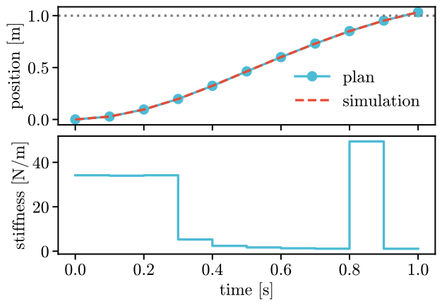
Solve_Succeeded 40 [34.2 34.  34.2  5.3  2.4  1.7  1.3  1.1 49.4  1.1]

Shooting(q0, horizon, nodes, ...) starts the plan at q0, over horizon seconds, with nodes nodes (one more than the intervals), and Cost(coordinate, weight, name=...) weighs the integral of the squared coordinate. The Ref target of the cost named reach is the input "reach.target" of each solve.

plan.steps[K] holds the stiffness of each of the 10 intervals, plan.steps[GOAL] the reference. The other Params of the plan stay as they are. Since the plan is the closed loop of a simulation, we can check it by running one. We hold the planned Params in each interval, and simulate with the same control step:

plant = vmc.sim.ModelPlant(robot, max_step=0.02)
controller = vmc.VMCController(vmc.compile(system))
controller.reset(0.0, plant.read())
q_run = [plant.q[0]]
for i in range(INTERVALS * SUBSTEPS):
    if i % SUBSTEPS == 0:
        plan.apply(controller, interval=i // SUBSTEPS)
    plant.write(controller.step(plant.t, plant.read()))
    plant.advance(0.02)
    q_run.append(plant.q[0])

The simulated motion follows the plan within 2e-07 mm: it is the same closed loop. The planned stiffness starts at 34 N/m, and the spring is first pulled to 1.26 m, beyond the goal, which gets the mass moving.

fig, (top, bottom) = plt.subplots(2, 1, sharex=True)
top.plot(plan.t, plan.q[:, 0], "o-", label="plan")
top.plot(plan.t, np.array(q_run)[::SUBSTEPS], "--", label="simulation")
top.axhline(1.0, color="gray", linestyle=":")
top.set_ylabel("position [m]")
top.legend(loc="lower right", fontsize=18)
bottom.step(plan.t, np.r_[plan.steps[K], plan.steps[K][-1]], where="post")
bottom.set_xlabel("time [s]")
bottom.set_ylabel("stiffness [N/m]");

Planning again at every step¶

MPC wraps the problem. It builds the program once, and every step solves it from the measured state, starting from the previous plan moved one interval on. It sets the Params of the plan on the controller through controller.set, and returns the jump this gave the controller’s energy, as the adaptation laws do:

mpc = opt.MPC(problem)  # the start and the Params that step become inputs


def run(mpc, seconds, level=None, cold=False, latency=0.0):
    """The mass under the controller; a plan every 5 control steps."""
    plant = vmc.sim.ModelPlant(robot, max_step=0.02)
    controller = vmc.VMCController(vmc.compile(system))
    if level is not None:
        controller = vmc.control.Tank(controller, level=level)
    controller.reset(0.0, plant.read())
    log = []
    for i in range(round(seconds / 0.02)):
        command = controller.step(plant.t, plant.read())
        if i % SUBSTEPS == 0:
            if cold:
                mpc.reset()  # forget the previous plan
            mpc.step(controller, plant.q, plant.v, latency=latency)
            tank = controller if level is not None else None
            log.append((plant.t, plant.q[0], mpc.result.iterations,
                        mpc.result.seconds,
                        tank.level if tank else 0.0,
                        tank.fraction if tank else 1.0))
        plant.write(command)
        plant.advance(0.02)
    return np.array(log)


warm = run(mpc, 3.0)

The controller moves first, and step changes its Params for the next control step. A plan that came late is applied as of the time it took (latency, in seconds, measured by default); here it is 0, as the simulation has no clock of its own. The target is an input of each solve (problem.parameter("reach.target") above), so a new one moves the goal while the controller runs: mpc.step(controller, q, v, references={"reach.target": [1.5]}).

fig, ax = plt.subplots()
ax.plot(warm[:, 0], warm[:, 1])
ax.axhline(1.0, color="gray", linestyle=":")
ax.set_xlabel("time [s]")
ax.set_ylabel("position [m]");

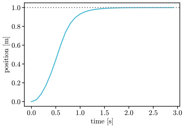
The mass arrives, 0.02 mm from the goal at the end. A plan took 5 ms on average. Starting each solve from the shifted previous plan took 408 iterations in all, against 660 when every solve started from the measured state alone (mpc.reset() forgets the plan).

Planning in a thread¶

On a robot with a real clock, a solve that takes several control periods must not hold the control loop. start plans in a thread from the measured state, and poll applies the plan once it is ready, as of the time that has passed since start, which is the real latency. This is a sketch of the loop: plant, running, q and v are yours:

while running:
    meas = plant.read()
    command = controller.step(meas.t, meas)
    plant.write(command)
    mpc.poll(controller)  # applies a plan that is ready, else nothing
    if not mpc.busy:
        mpc.start(controller, q, v)  # q and v: your estimate of the state

A solve lets the other threads run, so the loop keeps its rate. start does nothing while a plan is being made, and an error in the thread is raised by the next poll. Create the MPC after setting the problem’s solver and options, since it creates the solver then.

A tank pays for the changes¶

Changing the stiffness or the reference of a virtual spring gives the controller energy, or takes it. A tank is a budget for this: it applies a change as far as it can pay. TankBudget puts the budget into the plan, so that the plan does not ask for what the tank would cut. It tracks the tank’s level from the interval’s changes and from the energy that the controller’s dampers take back, and keeps it at least zero. MPC reads the level of the tank it controls at every step:

def tight(budget):
    """A tank of 0.05 J, with a plan that knows it or not."""
    p = opt.Problem(system, solver="ipopt-exact")
    p.add(opt.Shooting([0.0], 1.0, INTERVALS + 1, steps=[K, GOAL],
                       substeps=SUBSTEPS))
    p.add(opt.Effort(0.01))
    p.add(opt.Cost(x - target, 1.0, name="reach"))
    if budget:
        p.add(opt.TankBudget(0.05))  # [J]; MPC reads the level every step
    p.parameter("reach.target")
    return run(opt.MPC(p), 3.0, level=0.05)


budgeted, unaware = tight(True), tight(False)

fig, ax = plt.subplots()
ax.plot(budgeted[:, 0], budgeted[:, 5], label="plan with the budget")
ax.plot(unaware[:, 0], unaware[:, 5], label="plan without")
ax.set_xlabel("time [s]")
ax.set_ylabel("share of the change applied")
ax.legend(loc="center right", fontsize=18);

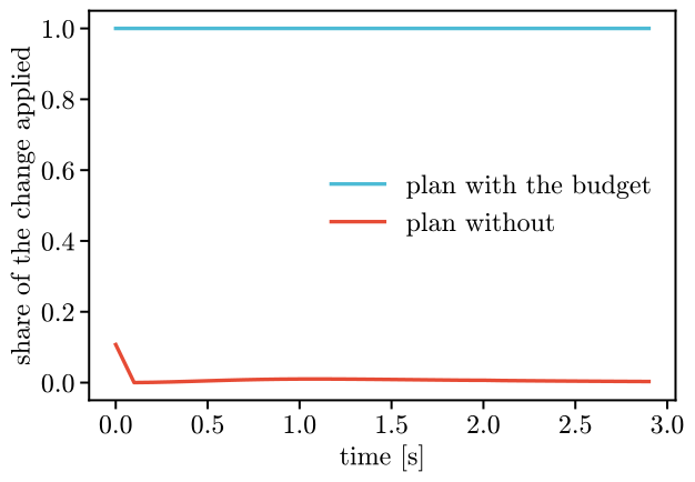
The tank holds 0.05 J, little for a spring of 2 N/m that must move a meter. The plan that knows the budget changes the Params in steps the tank pays in full (the share is 1 throughout), and the mass has moved 0.25 m by the end. The plan that does not asks for more, and the tank applies as little as 1.1e-04 of a change. Both keep the tank’s level above zero: the tank is what makes them safe. The term only lets the plan ask for what the tank can pay, instead of asking for more than it applies.

Real-time iteration¶

Solving to convergence at every step can take longer than a control period. The real-time iteration takes one iteration of sequential quadratic programming per step, from the shifted plan, and uses what it gives. The next step corrects it again:

fast = run(opt.MPC(problem, rti=True), 3.0)

Every plan is one iteration, and the mass ends 0.2 mm from the goal. A plan then is not an optimum, only a step towards it; plan.converged is false for it by design.

Solvers¶

Problem(system, solver=...) chooses a preset by name. opt.PRESETS lists them: "ipopt" (the default, with a quasi-Newton Hessian), "ipopt-exact" (exact Hessians, far fewer iterations on a shooting), "sqp" (CasADi’s SQP with the QP solver qrqp, any other with the qpsol option), "rti" and "fatrop". A preset needs its plugin in your CasADi build, and opt.solver.available(name) tells. All of them but "rti" find the same plan here:

import time

rows = {}
for name in opt.PRESETS:
    if not opt.solver.available(name):
        continue
    p = opt.Problem(system, solver=name)
    p.add(opt.Shooting([0.0], 1.0, INTERVALS + 1, steps=[K, GOAL],
                       substeps=SUBSTEPS))
    p.add(opt.Effort(0.01))
    p.add(opt.Cost(x - 1.0, 1.0, name="reach"))
    p.solve()  # builds the program and the solver
    start = time.perf_counter()
    result = p.solve()
    rows[name] = (result.iterations, result.cost,
                  1e3 * (time.perf_counter() - start), result.status)
for name, (iterations, cost, ms, _) in rows.items():
    print(f"{name:<12}{iterations:>4} iterations {ms:>6.1f} ms  "
          f"cost {cost:.4f}")

ipopt        165 iterations  106.9 ms  cost 0.5100
ipopt-exact   40 iterations   14.1 ms  cost 0.5099
sqp           93 iterations    9.8 ms  cost 0.5099
rti            1 iterations    0.7 ms  cost 0.5342
fatrop        46 iterations    8.5 ms  cost 0.5099

The default "ipopt" takes 165 iterations against 40 for "ipopt-exact", as its Hessian is approximate, and ends at an acceptable level; "rti" is one step from a cold start, so its plan is not the optimum.

Which QP solver the SQP presets use is the qpsol option, and not every one of CasADi’s suits a shooting. Tried on this problem with CasADi 3.7 and 3.8: qrqp (the default), qpoases and daqp find the same plan; proxqp stops at the iteration limit; hpipm needs the QP in stage order, and the program orders its variables by kind (all the \(q\), then all the \(v\)); ipqp needs a positive definite Hessian, which a shooting QP does not have, and fails; highs reports an optimum with a primal infeasibility above its own tolerance, and a looser tolerance does not help; osqp needs a newer OSQP library than the one in that CasADi build. Your build may differ: pass the name in qpsol and read plan.converged.

The library’s "fatrop" treats the program as one general problem, without the stages it was made for, so it does not scale with the horizon as FATROP can: for a long horizon take "ipopt-exact".

Good to know¶

• What is planned. Every Param named in steps takes one value per interval, between its bounds. The Params the problem frees take one value for the whole horizon, optimized again at every step and applied with the others. parameters are inputs of each solve: the goal, say, in step(..., references={...}).

• The control step. A plan is the closed loop of a simulation with a control step of horizon / (nodes - 1) / substeps. Make it the control period of your robot, or shorter. The integrator is the implicit step of vmc.sim.rollout by default, which is stable for stiff springs, or "rk4" for robots that are not stiff.

• Time. The controller’s time counts from the start of each plan.

• Virtual states. A controller with virtual states is planned from the state it runs in: give the Shooting a z0 (positions, then velocities), which mpc.step reads from controller.z at every step, and shifts with the plan. Without z0 the plan starts the controller afresh, as after a reset, and MPC refuses it.

• Applying a plan. mpc.interval is the interval that was applied, and mpc.result the whole plan. shift is how many intervals the horizon moves between two steps (1 by default).

• Limits. The warm start carries the plan, not the multipliers. The tank’s capacity is not planned. Sending a plan over a network is left to your own code: the library only turns a measurement into Params.

To tune a controller by trial runs instead, see Tuning, and to plan one motion offline with the same terms, see Optimizing a virtual mechanism.