Optimizing a virtual mechanism¶

In this tutorial we choose the stiffness of a virtual spring by optimization instead of by hand. We plan the motion of the soft arm together with the spring that drives it, using the arm’s own dynamics, and then check the plan by running the swap on the simulated arm.

The task¶

The hanging soft arm is held by a soft spring, the controller in place. We want to swap to a spring that pulls the tip to a target, with a force of at most 2 N, and to choose its stiffness: stiff enough to arrive, soft enough not to waste effort.

import numpy as np
import matplotlib.pyplot as plt
import virtualmodelcontrol as vmc
from virtualmodelcontrol import optimization as opt, viz
from virtualmodelcontrol.robots import helyx

arm = helyx.add_dynamics(helyx.arm("145-290-290"))  # hangs from its base
tip = arm.point(s=1.0)
target = [0.05, 0.02, 0.71]  # [m]

hold = vmc.Mechanism("hold")  # the controller in place
hold.add("drag", vmc.LinearSpring(tip - [0.01, 0.0, 0.70], 10.0))
hold.add("damp", vmc.LinearDamper(tip, 2.0))
hold.add("gravity", vmc.GravityCompensation(arm))
held = vmc.VirtualMechanismSystem(arm, hold)

stiffness = vmc.Param("stiffness", 20.0, bounds=(1.0, 300.0), scope="stage")
reference = vmc.Ref("reference", 3, target)  # where the spring pulls to
new = vmc.Mechanism("new")  # the controller to plan
spring = vmc.TanhSpring(tip - reference, stiffness, 2.0)  # [N/m], [N]
new.add("pull", spring)
new.add("damp", vmc.LinearDamper(tip, 2.0))
new.add("gravity", vmc.GravityCompensation(arm))
system = vmc.VirtualMechanismSystem(arm, new)

The stiffness is a Param with bounds, which the optimizer keeps to; scope="stage" makes it live in a compiled controller, so that controller.set can change it later. The planned motion starts at rest, so we first let the arm settle under the controller in place:

plant = vmc.sim.ModelPlant(arm)
settle = vmc.VMCController(vmc.compile(held))
vmc.sim.run(plant, settle, vmc.sim.SimClock(1 / 330), T=12.0)
q0 = plant.q.copy()  # the arm at rest under the spring in place

The problem¶

A Problem is a system whose Params we optimize, plus blocks. The Collocation block plans the motion of the closed loop from q0:

HORIZON, SWAP, NODES = 5.0, 2.0, 21  # [s], [s]


def build(free=(), parameters=(), terms=()):
    problem = opt.Problem(system)
    problem.add(opt.Collocation(q0, HORIZON, NODES, initial=held,
                                transition=SWAP))
    problem.free(*free)
    problem.parameter(*parameters)
    problem.add(opt.Effort(0.2))
    problem.add(opt.Cost(tip - target, t_from=SWAP, name="reach"))
    for term in terms:
        problem.add(term)
    return problem


problem = build(free=["new.pull.stiffness"])
plan = problem.solve()
print(plan.status, plan.iterations, plan.params, plan.costs)

Solve_Succeeded 18 {'new.pull.stiffness': array(124.46098225)} {'effort': 0.00024800707590755933, 'reach': 0.0004596531185837368}

The unknowns are the arm’s configuration, velocity and acceleration at 21 nodes, 0.25 s apart. The constraints are the arm’s dynamics at every node, written without inverting its mass matrix, and the trapezoid rule between the nodes, so the whole motion is solved at once and errors do not pile up along the horizon. The motion starts at rest where the arm is.

initial is the controller in place. Its torques fade out while the new ones fade in over transition, with the same blend as a swap, so the plan is what the swap executes.

free names the Params to optimize, with the names of problem.params: the mechanism, the element and the Param. It takes glob patterns, such as new.*.stiffness. Every Param not named stays at its value when the program is built. Two terms make the cost:

• Effort(0.2): 0.2 times the integral of the squared motor torques over the horizon;

• Cost(tip - target, t_from=SWAP): the integral of the squared distance of the tip to the target, from the end of the transition on: arrive, and stay.

Any library coordinate can stand where tip - target stands, and Bound keeps a coordinate within limits (see below).

The solver ended with Solve_Succeeded after 18 iterations. It chose a stiffness of 124 N/m. The cost has two parts, 2.48e-04 for the effort and 4.60e-04 for the distance to the target, and the largest violation of a constraint is 1e-06. plan also holds the motion at the nodes (t, q, v, a), the motor torques u and the weight blend of the new controller.

Is it a minimum?¶

To see it, we solve again with the stiffness fixed at each of several values. parameter makes a Param an input of each solve instead of a variable, so the program is built once and every solve is only the solver running again:

sweep = build(parameters=["new.pull.stiffness"])
ks = np.geomspace(5.0, 300.0, 25)
costs = np.array([sweep.solve({"new.pull.stiffness": k}).cost
                  for k in ks])

fig, ax = plt.subplots()
ax.semilogx(ks, 1e3 * costs, ".-", label="fixed stiffness")
ax.plot([k_found], [1e3 * plan.cost], "o", ms=10, label="optimized")
ax.set_xlabel("stiffness [N/m]")
ax.set_ylabel(r"cost [$10^{-3}$]")
ax.legend(loc="upper right", fontsize=18);

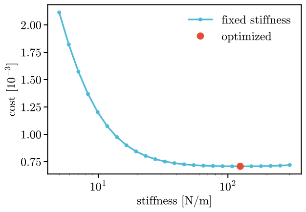
The optimized stiffness sits at the bottom of the curve, at the sweep’s own minimum (128 N/m on this grid). The bottom is flat: from 40 N/m up, the cost is at most 3 % above the minimum. Too soft a spring arrives late, and a stiffer one spends effort for little.

Checking the plan in simulation¶

The plan uses the same dynamics as the simulator, so running it should give the planned motion. apply puts the optimized Params into a controller, and a SwapController blends it in over the planned transition:

controller = vmc.VMCController(vmc.compile(system))
plan.apply(controller)  # the exact energy jump [J], 0 before its first step
swap = vmc.control.SwapController(
    vmc.VMCController(vmc.compile(held)))
swap.swap(controller, SWAP)

sim = vmc.sim.ModelPlant(arm, q0=q0)
log = vmc.sim.run(sim, swap, vmc.sim.SimClock(1 / 330), T=HORIZON)

kin = vmc.Kinematics(arm)
rows = log.arrays()
t = rows["t"].ravel()


def distance(q):  # [mm] from the tip to the target
    return 1e3 * np.linalg.norm(kin.position(q, 1.0) - target)


simulated = np.array([distance(q) for q in rows["q"]])
planned = np.array([distance(q) for q in plan.q])
at_nodes = np.interp(plan.t, t, simulated)

fig, ax = plt.subplots()
ax.plot(t, simulated, label="simulated swap")
ax.plot(plan.t, planned, "o", label="plan")
ax.axvline(SWAP, color="gray", linestyle=":")
ax.set_xlabel("time [s]")
ax.set_ylabel("tip to target [mm]")
ax.legend(loc="upper right", fontsize=18);

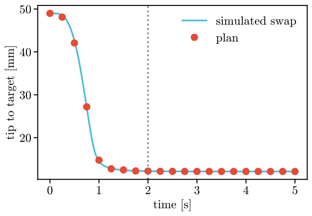
The tip starts 49 mm from the target and ends 12 mm from it: the spring is limited to 2 N and the arm pushes back. The simulated distance follows the plan within 0.5 mm at the nodes. The dotted line marks the end of the swap.

viz.animate(arm, log, "optimize.mp4", springs=[(1.0, target)], trace=1.0,
            invert=True)

Where the spring pulls to¶

The spring’s reference does not have to be the target. We make it a parameter and let the stiffness be optimized at each of the reference’s candidate points. search_references tries the points of a grid around the target, one reference at a time, and keeps the plan with the lowest cost among those that converged. The program is built once and every point is only another solve, warm-started from the best plan so far:

plan.apply(system)  # the system's stiffness is now the optimized one
search = build(free=["new.pull.stiffness"],
               parameters=["new.pull.reference"])
found = opt.search_references(
    search, {"new.pull.reference": target}, radius=0.06, step=0.06)

key = "new.pull.reference"
for c in found.candidates:
    offset = 1e3 * (np.array(c["references"][key]) - target)  # [mm]
    cost = np.nan if c["cost"] is None else c["cost"]  # None: not converged
    print(f"{offset.round().astype(int).tolist()} mm  "
          f"{c['status']:<26} {cost:.2e}")

[0, 0, 0] mm  Solve_Succeeded            7.08e-04
[-60, 0, 0] mm  Solve_Succeeded            1.19e-02
[0, -60, 0] mm  Solved_To_Acceptable_Level 1.18e-02
[0, 0, -60] mm  Solve_Succeeded            7.06e-04
[0, 0, 60] mm  Solve_Succeeded            8.28e-04
[0, 60, 0] mm  Solved_To_Acceptable_Level 1.17e-02
[60, 0, 0] mm  Solved_To_Acceptable_Level 1.15e-02

Radius and step are in meters: a radius of 6 cm and a step of 6 cm give the target and its six neighbors. The status says how each solve ended: an acceptable level counts as converged, and a point that did not converge has no cost. The best reference lies 60 mm from the target along z, and it lowers the cost by 0.2 %, with a stiffness of 124 N/m: for this task the target is already a good reference. Moving it sideways costs at least 16 times more. found.result is the plan, found.references the point that gave it, and found.candidates every point tried.

Where the arm rests¶

A plan spends its time getting there. When only the pose at rest matters, Equilibrium takes the place of Collocation: it solves for a configuration where the controller’s torques balance the arm’s own forces, with the same terms and the same free Params. The spring is the optimized one from above, and nothing is free yet:

def miss(rest):  # [mm] from the tip at rest to the target
    return 1e3 * np.linalg.norm(kin.position(rest.q[0], 1.0) - target)


rest = opt.Problem(system)
rest.add(opt.Equilibrium(q0))  # q0 is the first guess
rest.add(opt.Cost(tip - target, name="miss"))
there = rest.solve()

rest.free("new.pull.reference")  # now ask for the best reference
nearest = rest.solve()

The arm rests 12.1 mm from the target, where the plan ended, and the solve took 23 ms. With the reference free, the nearest it can rest is 11.6 mm: the spring saturates at 2 N, so no reference pulls harder. A Bound holds at the equilibrium too. Cost and Effort weigh its single node once.

Limits¶

Bound keeps a coordinate within limits at every node but the first, which is the fixed start. Here the tip must stay below 30 mm in x, and the stiffness has to give way:

wall = opt.Bound(tip[0], upper=0.03, name="wall")
capped = build(free=["new.pull.stiffness"], terms=[wall]).solve()
x_free = 1e3 * np.array([kin.position(q, 1.0)[0] for q in plan.q])
x_capped = 1e3 * np.array([kin.position(q, 1.0)[0] for q in capped.q])

fig, ax = plt.subplots()
ax.plot(plan.t, x_free, label="free")
ax.plot(capped.t, x_capped, label="with the bound")
ax.axhline(30.0, color="gray", linestyle=":")
ax.set_xlabel("time [s]")
ax.set_ylabel("tip x [mm]")
ax.legend(loc="lower right", fontsize=18);

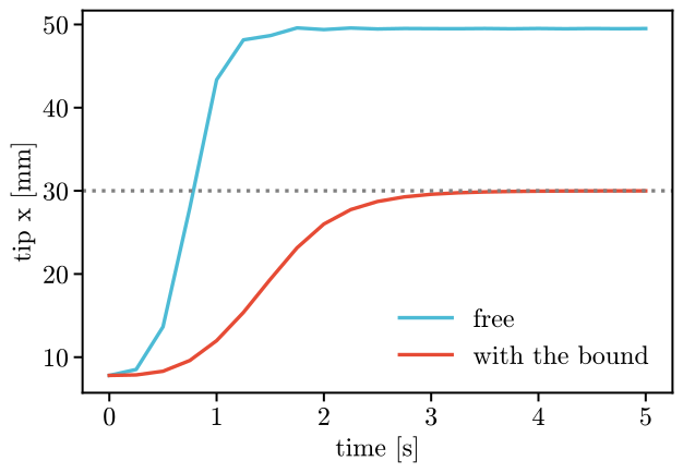
Without the bound the tip goes to 50 mm; with it the tip stops at the limit, and the optimizer picks a softer spring, 4.6 N/m. The Bound’s coordinate can be anything the library knows: a joint, a distance to a sphere or a plane (see Contact), the sum of several, or your own vmc.Custom.

Good to know¶

• Scales. The solver works on q, v and a divided by Collocation(scales=(s_q, s_v, s_a)), the typical sizes of the three, (1, 1, 1) by default. Scaling does not change the problem, but it changes the solver’s path, and a problem with several local optima can end in a different one: try other scales, or other starting values, when a plan looks poor.

• Schemes. Collocation(scheme="hermite-simpson") integrates to fourth order instead of second. It adds the acceleration at the middle of every interval to the unknowns, so each node costs more, but far fewer nodes give the same agreement with a simulation.

• Starting values. The free Params start at their current values, and the warm_start argument of solve takes a previous Result (or a dict of q, v, a and params) to start from its plan.

• What is rebuilt. The values of the free Params and of the parameters, and the bounds of the free Params, are read at every solve. Everything else (a gain, a limit such as the 2 N here) is folded in when the program is built: to change it, make it free or a parameter, or build a new Problem.

• Options. Problem(system, solver="ipopt-exact") takes a preset (the others are in Model predictive control), and options={...} overrides its defaults: IPOPT’s are listed in opt.IPOPT, and any other IPOPT option is accepted, such as "ipopt.max_wall_time". Changing problem.options later makes the next solve create the solver again.

• Status. plan.converged is true for a solution and for an acceptable one; read plan.status and plan.violation before trusting a plan.

• Your own term. Subclass opt.Term and write cost(trajectory) and constraints(trajectory), and coordinates() to list the coordinates it uses; trajectory.coordinate(c) gives a coordinate and its rate at every node.

• Stopping. progress(iteration, cost, params, q) of solve is called at every iteration; return True from it to stop the solve there (the status is User_Requested_Stop).

• A larger plant. Problem(system, plant=robot) takes the dynamics from robot while the controller stays written for other coordinates (the two cranks of the turtle, a robot’s motors): it reads the plant’s motors as it does in a simulation. q0 and the terms are in the plant’s coordinates, and a plan equals the simulation step for step (Crawl with a flywheel shows it on the crawler).

• Limits. Collocation needs the robot’s configuration in a flat space (every robot template here does); Shooting also plans a floating body, with unit quaternions at its nodes.

More plans: around an obstacle, and which fields to keep, and a periodic motion and a controller with virtual states.

To change a running controller within an energy budget, see Energy and passivity, and to tune one by trial runs instead of a plan, see Tuning. To plan again at every step from the measured state, with multiple shooting and a tank, see Model predictive control, which also has the other solver presets.